

GWB#
Suite of various geospatial image analysis tools
This article provides usage instructions for the image analysis module GuidosToolbox Workbench (GWB), implemented as a Jupyter dashboard on the SEPAL platform (for more information on GWB), see https://forest.jrc.ec.europa.eu/en/activities/lpa/gwb/).
Introduction#
In 2008, GuidosToolbox (GTB)) (Vogt and Riitters, 2017) was developed as a graphical user interface (GUI) to the Morphological Spatial Pattern Analysis (MSPA) of raster data (Soille and Vogt, 2009).
GTB has since been enhanced with numerous modules for analysis of landscape objects, patterns and networks, as well as specialized modules for assessing fragmentation and restoration.
GWB provides the most popular GTB modules as a set of command-line applications for 64bit Linux systems.
In this article, we describe the implementation of GWB on the SEPAL platform as a Jupyter dashboard based on the GWB CLI tool.
Presentation#
To launch the app, register to SEPAL.
Then, navigate to the SEPAL Apps dashboard (purple wrench icon in the left pane).
Finally, search for and select GWB ANALYSIS.
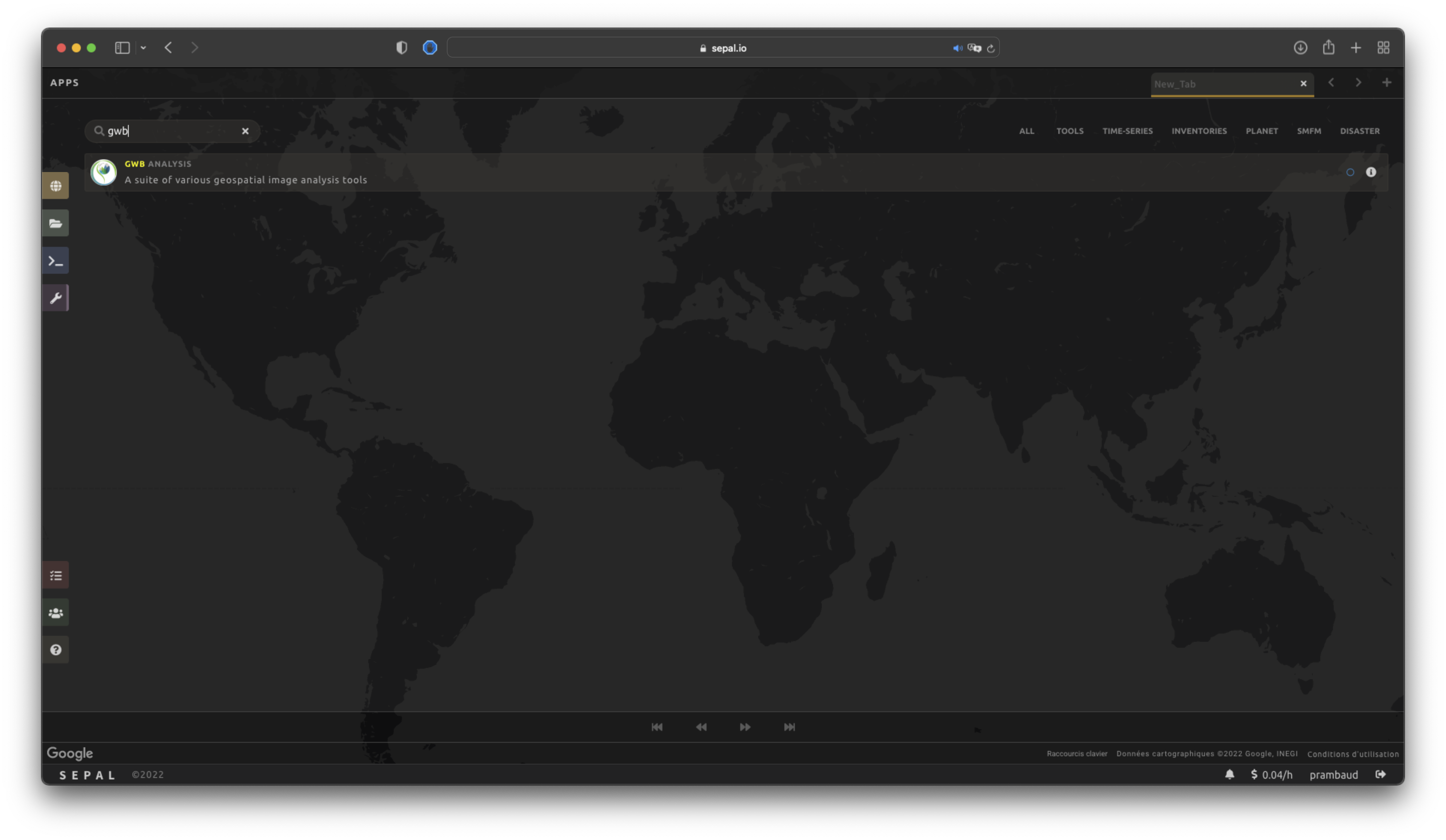
The application should launch itself and display the About section.
Select the tool you want to use.
Note
If this is the first time you have used the app, you will see the following pop-up window:
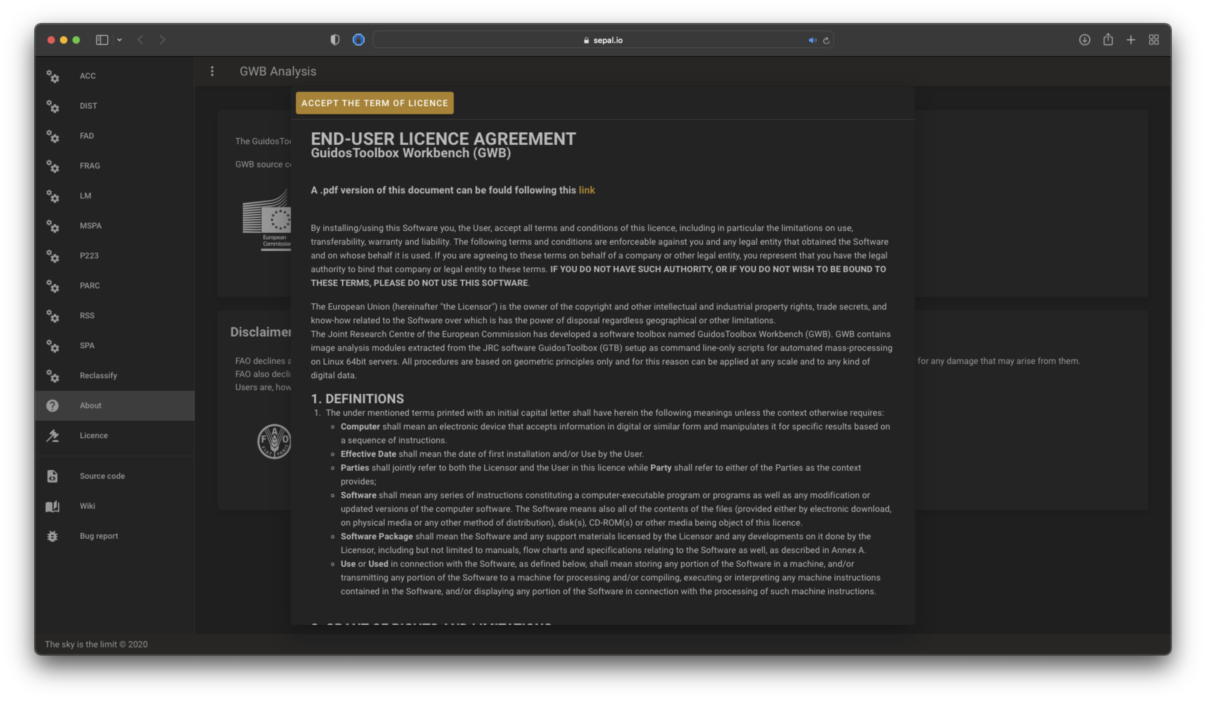
This licence needs to be accepted to use the GWB modules. It is also available in the Licence section of the app.
If you don’t want to accept the licence, close the app tab.
Usage#
General structure#
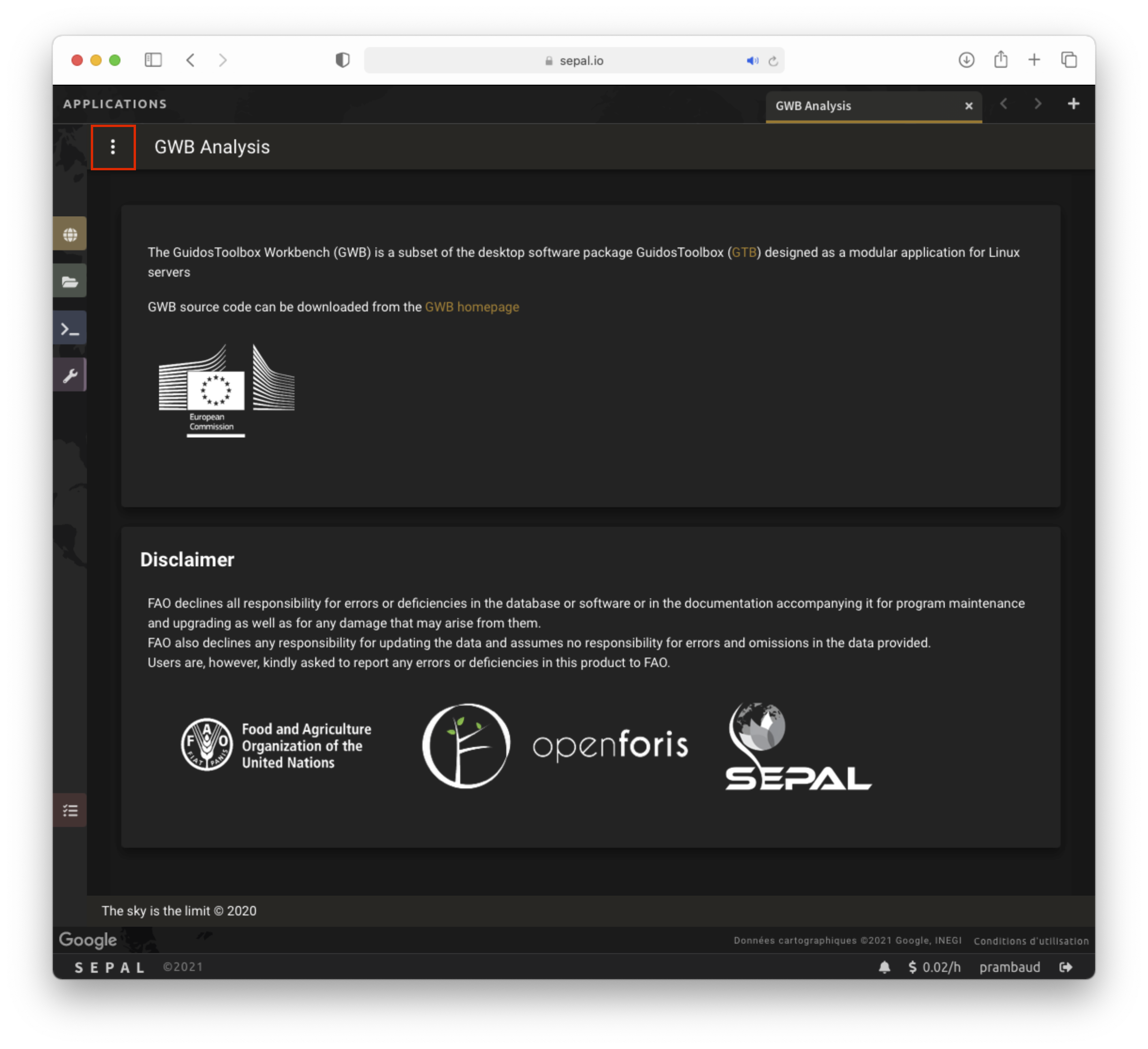
The application is structured as follows:
On the left, there is a navigation drawer that you can open and close using the (upper-left side of the window).
Tip
On small devices such as tablets or phones, the navigation drawer will be hidden by default. Select the (upper-left side) to display the full extent of the app.
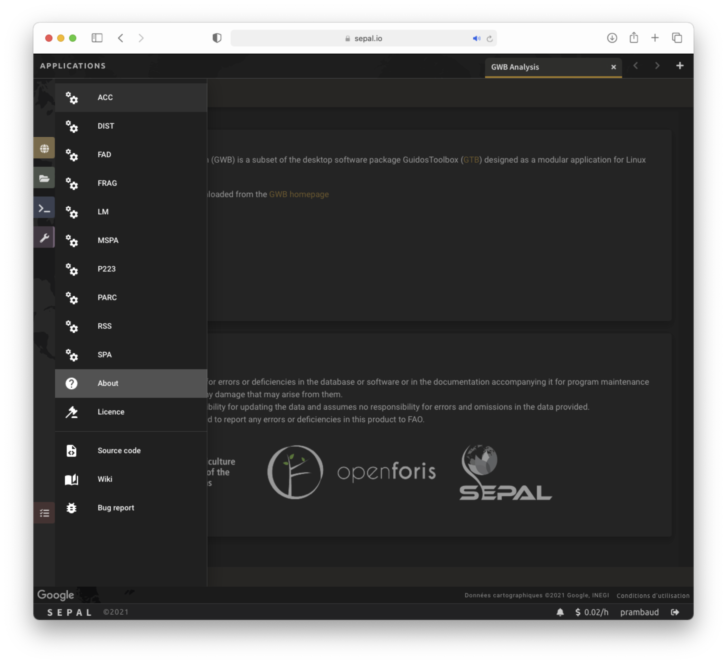
Each name in the list corresponds to one GWB module, presented separately in the following sections. By selecting a name, the panes relative to the function will be displayed.
Attention
All GWB modules require categorical raster input maps in data type unsigned bytes (8bit), with discrete integer values within [0, 255] bytes. Any other data format will cause an error.
Launch a module#
For all modules, the first step is sanitizing the image provided by the user and changing the band values according to module requirements.
Then, select the parameters associated with the selected module and run it by selecting the final button.
In the next section, each module and its specificities will be described.
Note
The module_results folder is dedicated to producing data, not saving them. Once created, no binary image using the same name can be produced. If you’re running the same analysis with different parameters, you can safely reuse the same one; if not, please delete or move the previous image before running. A warning message will be displayed in the application.
Modules#
Each module is presented individually in this article. You can directly jump to the module of interest by selecting the related link under the Modules section in the right pane of this page – the documentation will guide you through the respective processing steps.
Accounting (ACC)#
This module will conduct the Accounting analysis. Accounting will label and calculate the area of all foreground objects. The results are spatially explicit maps and tabular summary statistics. Details on the methodology and input/output options can be found in the Accounting product sheet.
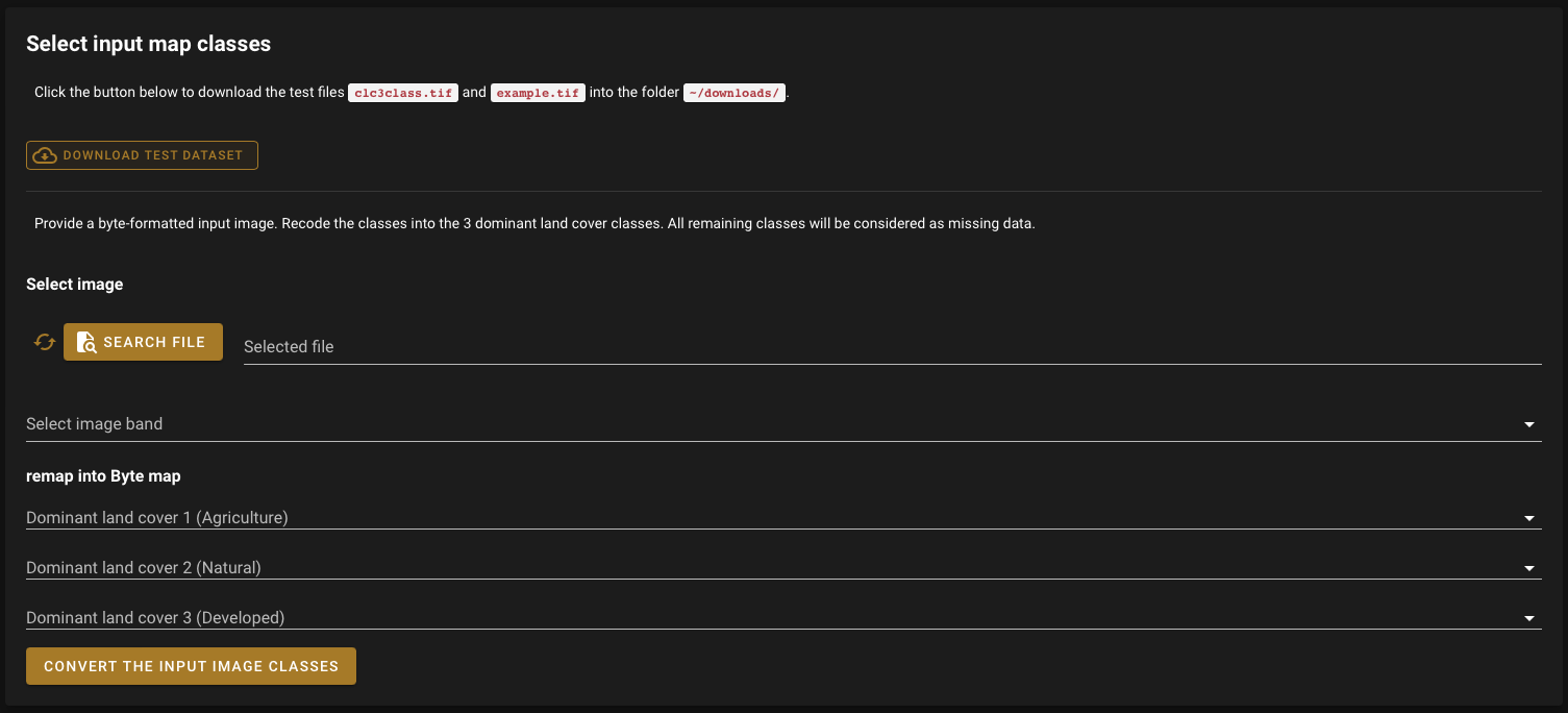
Set up the input image#
Tip
You can use the default dataset to test the module. Select the Download test dataset button on the top of the second pane to add the following files to your downloads folder:
example.tif: 0 bytes - Missing, 1 byte - Background, 2 bytes - Foregroundclc3class.tif: 1 byte - Agriculture, 2 bytes - Natural, 3 bytes - Developed
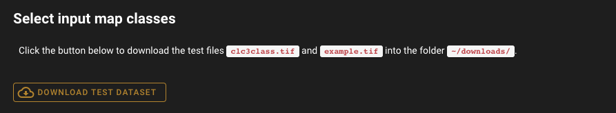
Once the files are downloaded, follow the normal process using the downloads/example.tif file (two classes).
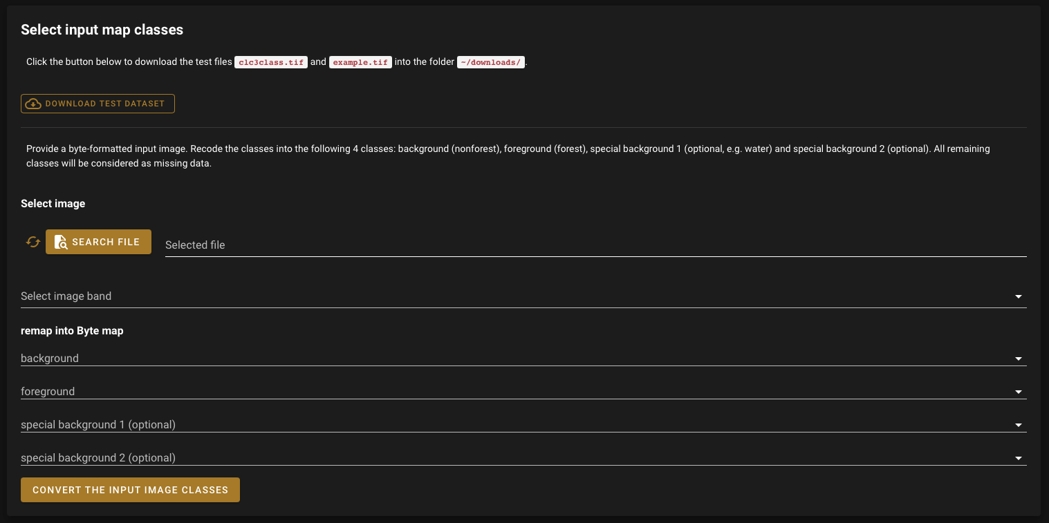
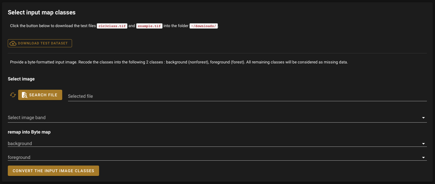
The first step requires reclassifying your image. Using the Reclassifying pane, select your image in your SEPAL folders.
Attention
If the image is on your local computer and not in your SEPAL folders, see Exchange files with SEPAL.
The dropdown menus will list the discrete values of your raster input image.
Select each class in your image and place them in one of the following categories:
background
foreground
special background 1 (optional)
special background 2 (optional)
Every class that is not set to a reclassifying category will be considered “missing data” (0 byte).
Tip
For forest analysis, set Forest as foreground and all other classes as background. If you specify a special background, it will be treated separately in the analysis (e.g. water, buildings).
Select the parameters#
You will need to select parameters for your computation:

Note
These parameters can be used to perform the default computation:
foreground connectivity: 8
spatial pixel resolution: 25
area thresholds: 200 2000 20000 100000 200000
option: default
big3pink: True
Foreground connectivity#
This sets the foreground connectivity of your analysis. Specifically:
8 neighbours (default) will use every pixel in the vicinity (including diagonals)
4 neighbours will only use the vertical and horizontal ones

Spatial pixel resolution#
Set the spatial pixel resolution of your image (in metres). It is only used for the summary.
Area thresholds#
Set up to five area thresholds (measured in pixels).
Options#
Two computation options are available:
stats + image of viewport (default)
stats + images of ID, area, viewport (detailed)
Big3pink#
Two options are available:
do not highlight the three largest objects (False)
show the three largest objects in pink color (True)
Run the analysis#
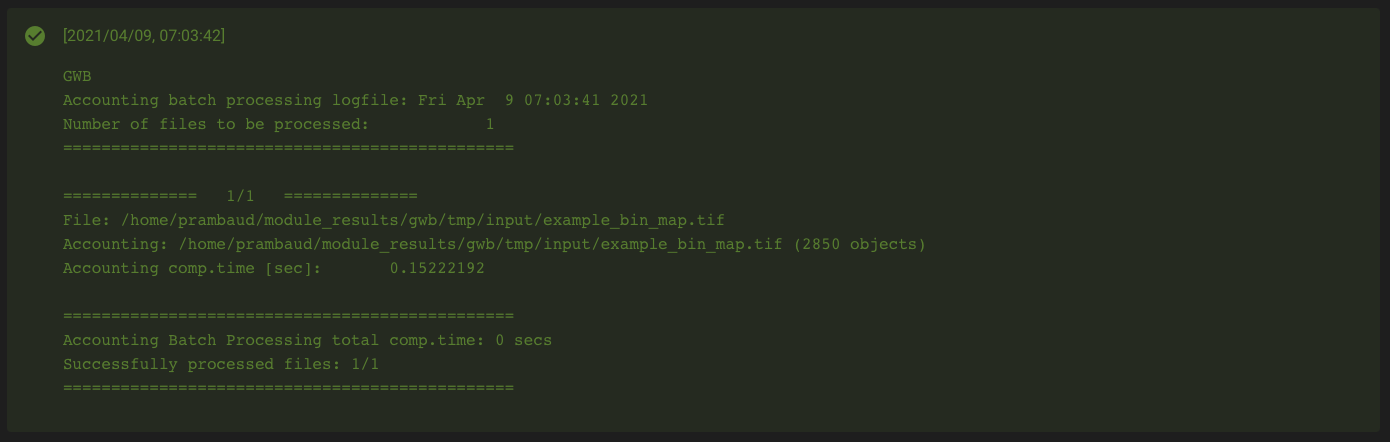
Once your parameters are set, launch the analysis. The blue rectangle will display information about the computation. Upon completion, it will turn green and display the Computation log.
The resulting files are stored in the folder module_results/gwb/acc/. For example:
<raster_name>_bin_map.tif<raster_name>_bin_map_acc.tif<raster_name>_bin_map_acc.csv<raster_name>_bin_map_acc.txt
Attention
If the rectangle turns red, carefully read the information in the log. For example, your current instance may be too small to handle the file you want to analyse. In this case, close the app, open a bigger instance and run your analysis again.
Here is the result of the computation using the default parameters on the example.tif file.

Euclidean Distance (DIST)#
This module will conduct the Euclidean Distance analysis. Each pixel will show the shortest distance to the foreground boundary. Pixels inside a foreground object have a positive distance value while background pixels have a negative distance value. The results are spatially explicit maps and tabular summary statistics.
Details on the methodology and input/output options can be found in the Distance product sheet.
Set up the input image#
Tip
You can use the default dataset to test the module. Select the Download test dataset button on the top of the second pane to add the following files to your downloads folder:
example.tif: 0 bytes - Missing, 1 byte - Background, 2 bytes - Foregroundclc3class.tif: 1 byte - Agriculture, 2 bytes - Natural, 3 bytes - Developed
Once the files are downloaded, follow the normal process using the downloads/example.tif file (two classes).
The first step requires reclassifying your image. Using the Reclassifying pane, select the image in your SEPAL folder.
Attention
If the image is on your local computer and not in your SEPAL folders, see Exchange files with SEPAL.
The dropdown menus will list the discrete values of your raster input image. Select each class in your image and place them in one of the following categories:
background
foreground
Every class that is not set to a reclassifying category will be considered “missing data” (0 bytes).
Tip
For forest analysis, set Forest as foreground and all other classes as background.
Select the parameters#
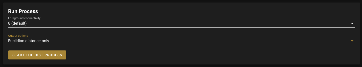
You will need to select parameters for your computation:
Note
These parameters can be used to perform the default computation:
Foreground connectivity: 8
Options: Euclidian Distance only
Foreground connectivity#
This sets the foreground connectivity of your analysis. Specifically:
8 neighbors (default) will use every pixel in the vicinity (including diagonals)
4 neighbors will only use the vertical and horizontal one
Options#
Two computation options are available:
compute the Euclidian Distance only
compute the Euclidian Distance and the Hysometric Curve
Run the analysis#
Once your parameters are set, launch the analysis. The blue rectangle will display information about the computation. Upon completion, it will turn green and display the Computation log.
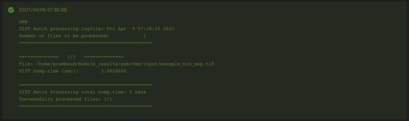
The resulting files are stored in the folder module_results/gwb/dist/. For example:
<raster_name>_bin_map.tif<raster_name>_bin_map_dist.tif<raster_name>_bin_map_dist.txt<raster_name>_bin_map_dist_hist.png<raster_name>_bin_map_dist_viewport.tif
Attention
If the rectangle turns red, carefully read the information in the log. For example, your current instance may be too small to handle the file you want to analyse. In this case, close the app, open a bigger instance and run your analysis again.
Here is the result of the computation using the default parameters on the example.tif file.


Forest area density (FAD)#
This module will conduct the Fragmentation analysis at five fixed observation scales.
Since forest fragmentation is scale-dependent, fragmentation is reported at five observation scales, allowing different observers to make their own choice about scales and threshold of concern.
The change of fragmentation across different observation scales provides additional information of interest.
Fragmentation is measured by determining forest area density (FAD) within a shifting, local neighbourhood. It can be measured at pixel or patch level. The results are spatially explicit maps and tabular summary statistics (details on the methodology and input/output options can be found in the Fragmentation product sheet).
Set up the input image#
Tip
You can use the default dataset to test the module. Select the Download test dataset button on the top of the second pane, which will add the following files to your downloads folder:
example.tif: 0 bytes - Missing, 1 byte - Background, 2 bytes - Foregroundclc3class.tif: 1 byte - Agriculture, 2 bytes - Natural, 3 bytes - Developed
Once the files are downloaded, follow the normal process using the downloads/example.tif file (two classes).
The first step requires reclassifying your image. Using the Reclassifying pane, select the image in your SEPAL folders.
Attention
If the image is on your local computer but not in your SEPAL folders, see Exchange files with SEPAL.
The dropdown menus will list the discrete values of your raster input image. Select each class in your image and place them in one of the following categories:
background
foreground
special background 1 (optional)
special background 2 (optional)
Every class that is not set to a reclassifying category will be considered “missing data” (0 bytes).
Tip
For forest analysis, set Forest as foreground and all other classes as background. If you specify a special background, it will be treated separately in the analysis (e.g. water, buildings).
Attention
Special background 2 is the non-fragmenting background (optional). For details, see the Fragmentation product sheet.
Select the parameters#
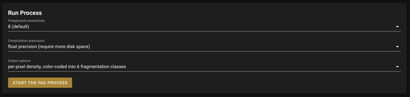
You will need to select parameters for your computation:
Note
These parameters can be used to perform the default computation:
Foreground connectivity: 8
Computation precision: float-precision
Options: per-pixel density, color-coded into 6 fragmentation classes (FAD)
Foreground connectivity#
This sets the foreground connectivity of your analysis:
8 neighbours (default) will use every pixel in the vicinity (including diagonals)
4 neighbours only will use the vertical and horizontal one
Computation precision#
Set the precision used to compute your image. Float precision (default) will give more accurate results compared to Rounded byte, but requires more computing resources and disk space.
Options#
Three computation options are available:
FAD: per-pixel density, color-coded into 6 fragmentation classes
FAD-APP2: average per-patch density, color-coded into 2 classes
FAD-APP5: average per-patch density, color-coded into 5 classes
Run the analysis#
Once your parameters are all set, you can launch the analysis. The blue rectangle will display information about the computation. Upon completion, it will turn green and display the Computation log.

The resulting files are stored in the folder module_results/gwb/fad/. For example:
<raster_name>_bin_map.tif<raster_name>_bin_map_fad_<class_number>.tif<raster_name>_bin_map_fad_barplot.png<raster_name>_bin_map_fad_mscale.csv<raster_name>_bin_map_fad_mscale.tif<raster_name>_bin_map_fad_mscale.txt<raster_name>_bin_map_fad_mscale.sav
Attention
If the rectangle turns red, carefully read the information in the log. For example, your current instance may be too small to handle the file you want to analyse. In this case, close the app, open a bigger instance, and run your analysis again.
Here is the result of the computation using the default parameters on the example.tif file.


Fragmentation (FRAG)#
This module will conduct the Fragmentation analysis at a user-selected observation scale.
This module and its option are similar to fad, but allow the user to specify a single (or multiple) specific observation scale. The results are spatially explicit maps and tabular summary statistics. Details on the methodology and input/output options can be found in the Fragmentation product sheet.
Set up the input image#
Tip
You can use the default dataset to test the module. Select the Download test dataset button on the top of the second pane, which will add the following files to your downloads folder:
example.tif: 0 bytes - Missing, 1 byte - Background, 2 bytes - Foregroundclc3class.tif: 1 byte - Agriculture, 2 bytes - Natural, 3 bytes - Developed
Once the files are downloaded, follow the normal process using the downloads/example.tif file (two classes).
The first step requires reclassifying your image. Using the Reclassifying pane, select the image in your SEPAL folders.
Attention
If the image is on your local computer but not in your SEPAL folders, see Exchange files with SEPAL.
The dropdown menus will list the discrete values of your raster input image. Select each class in your image and place them in one of the following categories:
background
foreground
special background 1 (optional)
special background 2 (optional)
Every class that is not set to a reclassifying category will be considered “missing data” (0 byte).
Tip
For forest analysis, set Forest as foreground and all other classes as background. If you specify a special background, it will be treated separately in the analysis (e.g. water, buildings).
Attention
Special background 2 is the non-fragmenting background (optional). For details, see the Fragmentation product sheet.
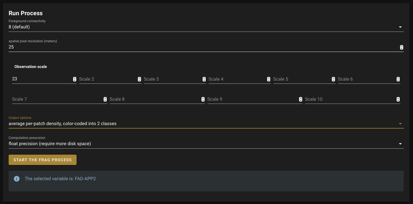
Select the parameters#
You will need to select parameters for your computation:
Note
These parameters can be used to perform the default computation:
Foreground connectivity: 8
Spatial pixel resolution: 25
Computation precision: float-precision
Window size: 23
Options: fragmentation at pixel- or patch- level with various number of color-coded classes
Foreground connectivity#
This sets the foreground connectivity of your analysis:
8 neighbours (default) will use every pixel in the vicinity (including diagonals)
4 neighbours will only use the vertical and horizontal one
Spatial pixel resolution#
Set the spatial pixel resolution of your image in metres. This is only used for the summary.
Window size#
Set up to 10 observation window sizes (in pixels).
Options#
Four computation options are available:
FOS5: per-pixel density, color-coded into 5 fragmentation classes
FOS6: per-pixel density, color-coded into 6 fragmentation classes
FOS-APP2: average per-patch density, color-coded into 2 classes
FOS-APP5: average per-patch density, color-coded into 5 classes
Run the analysis#
Once your parameters are all set, you can launch the analysis. The blue rectangle will display information about the computation. Upon completion, it will turn green and display the Computation log.

The resulting files are stored in the folder module_results/gwb/frag/. For example:
<raster_name>_bin_map.tif<raster_name>_bin_map_frag_fad-<option>_<class>.tif<raster_name>_bin_map_frag.csv<raster_name>_bin_map_frag.txt<raster_name>_bin_map_frag.tif
Attention
If the rectangle turns red, carefully read the information in the log. For example, your current instance may be too small to handle the file you want to analyse. In this case, close the app, open a bigger instance and run your analysis again.
Here is the result of the computation using the FAD-APP2 option on the example.tif file:

Landscape mosaic (LM)#
This module will conduct the Landscape mosaic analysis at a user-selected observation scale.
The Landscape mosaic measures land cover heterogeneity, or human influence, in a tri-polar classification of a location accounting for the relative contributions of the three land cover types (Agriculture, Natural, Developed) in the area surrounding that location.
The results are spatially explicit maps and tabular summary statistics. Details on the methodology and input/output options can be found in the Landscape mosaic product sheet.
Set up the input image#
Tip
You can use the default dataset to test the module. Select the Download test dataset button on the top of the second pane, which will add the following files to your downloads folder:
example.tif: 0 bytes - Missing, 1 byte - Background, 2 bytes - Foregroundclc3class.tif: 1 byte - Agriculture, 2 bytes - Natural, 3 bytes - Developed
Once the files are downloaded, follow the normal process using the downloads/clc3class.tif file (three classes).
The first step requires reclassifying your image. Using the Reclassifying pane, select the image in your SEPAL folders.
Attention
If the image is on your local computer and not in your SEPAL folders, see Exchange files with SEPAL.
The dropdown menus will list the discrete values of your raster input image. Select each class in your image and place them in one of the following categories:
dominant land cover 1 (Agriculture)
dominant land cover 2 (Natural)
dominant land cover 3 (Developed)
Every class that is not set to a reclassifying category will be considered “missing data” (0 bytes).
Select the parameters#
You will need to select parameters for your computation:

Note
This parameter can be used to perform the default computation:
window size: 23
Window size#
Set the square window size (in pixels). It should be an odd number in [3, 5, …501], with \(kdim\) being the window size, which is related to the observation scale by the following formula:
Also note the following:
\(obs_scale\) in hectares
\(pixres\) in metres
\(kdim\) in pixels
Run the analysis#
Once your parameters are all set, you can launch the analysis. The blue rectangle will display information about the computation. Upon completion, it will turn green and display the Computation log.

The resulting files are stored in the folder module_results/gwb/lm/. For example:
<raster_name>_bin_map.tif<raster_name>_bin_map_lm_23.tif<raster_name>_bin_map_lm_23_103class.tif<raster_name>_bin_map_heatmap.csv<raster_name>_bin_map_heatmap.png<raster_name>_bin_map_heatmap.savheatmap_legend.pnglm103class_legend.png
Attention
If the rectangle turns red, carefully read the information in the log. For example, your current instance may be too small to handle the file you want to analyse. In this case, close the app, open a bigger instance and run your analysis again.
Here is the result of the computation using the default parameters on the clc3classes.tif file:


Morphological Spatial Pattern Analysis (MSPA)#
Attention
If you are considering using the MSPA module, keep in mind that the result provides a lot of information (up to 25 classes). The alternative module GWB_SPA provides a similar, yet simplified assessment with up to six classes only. Both modules describe morphological features of foreground objects. While MSPA may address certain features of fragmentation, a more comprehensive assessment of fragmentation is obtained with the dedicated fragmentation modules: GWB_FRAG or GWB_FAD.
This module will conduct MSPA analysis shape and connectivity, as well as conduct a segmentation of foreground patches in up to 25 feature classes. The results are spatially explicit maps and tabular summary statistics. Details on the methodology and input/output options can be found in the Morphology product sheet.
Set up the input image#
Tip
You can use the default dataset to test the module. Select the Download test dataset button on the top of the second pane, which will add the following files to your downloads folder:
example.tif: 0 byte - Missing, 1 byte - Background, 2 bytes - Foregroundclc3class.tif: 1 byte - Agriculture, 2 bytes - Natural, 3 bytes - Developed
Once the files are downloaded, follow the normal process using the downloads/example.tif file (two classes).
The first step requires reclassifying your image. Using the Reclassifying pane, select the image in your SEPAL folders.
Attention
If the image is on your local computer and not in your SEPAL folders, see Exchange files with SEPAL.
The dropdown menus will list the discrete values of your raster input image. Select each class in your image and place them in one of the following categories:
background
foreground
Every class that is not set to a reclassifying category will be considered “missing data” (0 bytes).
Tip
For forest analysis, set Forest as foreground and all other classes as background.
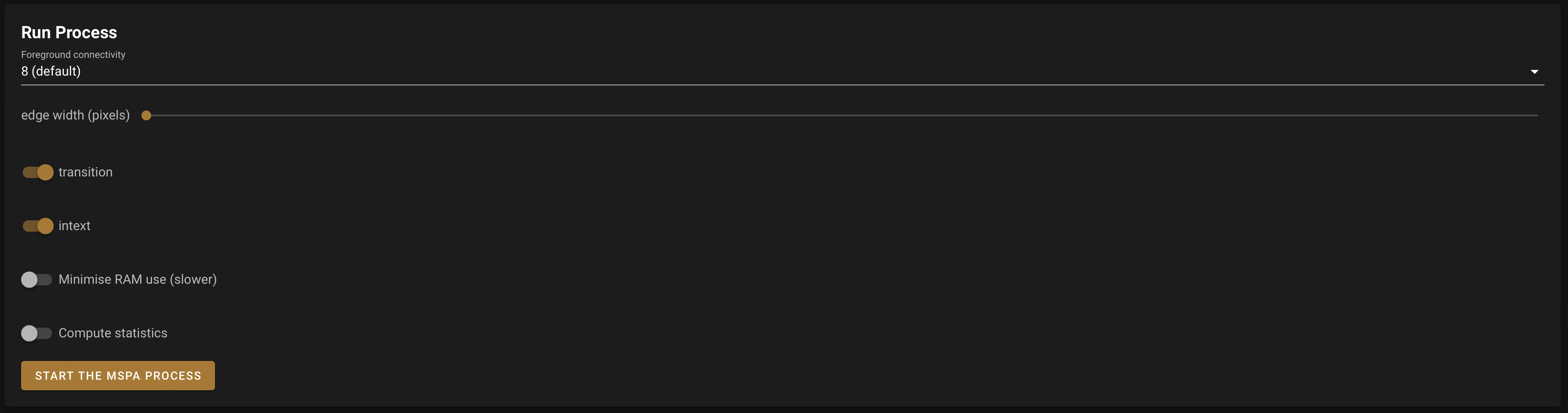
Select the parameters#
You will need to select parameters for your computation:
Note
These parameters can be used to perform the default computation:
Foreground connectivity: 8 (default)
Edge width: 1
Transition: True
Intext: True
Disk: False
Statistics: False
Foreground connectivity#
This sets the foreground connectivity of your analysis:
8 neighbours (default) will use every pixel in the vicinity (including diagonals)
4 neighbours will only use the vertical and horizontal one
Edge width#
Define the width (measured in pixels) of the core-boundaries (edges and perforations).
Transition#
Select if you want to show transition pixels, where connecting pathways go through edges/perforations (transition=1 (true), default) or not (transition=0).
Intext#
Select if you want to distinguish MSPA classes and holes laying within core objects (intext=1 (true), default) or not (intext=0).
Disk#
Select if you want to process with minimum RAM usage (disk=0 (false), default) or not (disk=1 (true) requires 20% less RAM but +40% processing time).
Statistics#
Select if you want to calculate summary statistics (statistics=0 (false), default) or (statistics=1 (true) +10% processing time)
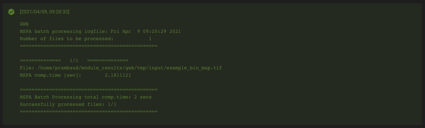
Run the analysis#
Once your parameters are set, you can launch the analysis. The blue rectangle will display information about the computation. Upon completion, it will turn green and display the computation log.
The resulting files are stored in the folder module_results/gwb/mspa/. For example:
<raster_name>_bin_map.tif<raster_name>_bin_map_<4 params>.tif<raster_name>_bin_map_<4 params>.txt
Attention
If the rectangle turns red, carefully read the information in the log. For example, your current instance may be too small to handle the file you want to analyse. In this case, close the app, open a bigger instance and run your analysis again.
Here is the result of the computation using the default parameters on the example.tif file.


Density, Contagion or Adjacency Analysis (P223)#
This module will conduct the Density (P2), Contagion (P22) or Adjacency (P23) analysis of foreground (FG) objects at a user-selected observation scale (Riitters et al., 2000).
The results are spatially explicit maps and tabular summary statistics.
The classification is determined by measurements of forest amount (P2) and connectivity (P22) within the neighbourhood that is centred on a subject forest pixel. P2 is the probability that a pixel in the neighbourhood is forest; P22 is the probability that a pixel next to a forest pixel is also forest.
Set up the input image#
Tip
You can use the default dataset to test the module. Select the Download test dataset button on the top of the second pane, which will add the following files to your downloads folder:
example.tif: 0 byte - Missing, 1 byte - Background, 2 bytes - Foregroundclc3class.tif: 1 byte - Agriculture, 2 bytes - Natural, 3 bytes - Developed
Once the files are downloaded, follow the normal process using the downloads/example.tif file (two classes).
The first step requires reclassifying your image. Using the Reclassifying pane, select the image in your SEPAL folders.
Attention
If the image is on your local computer but not in your SEPAL folders, see Exchange files with SEPAL.
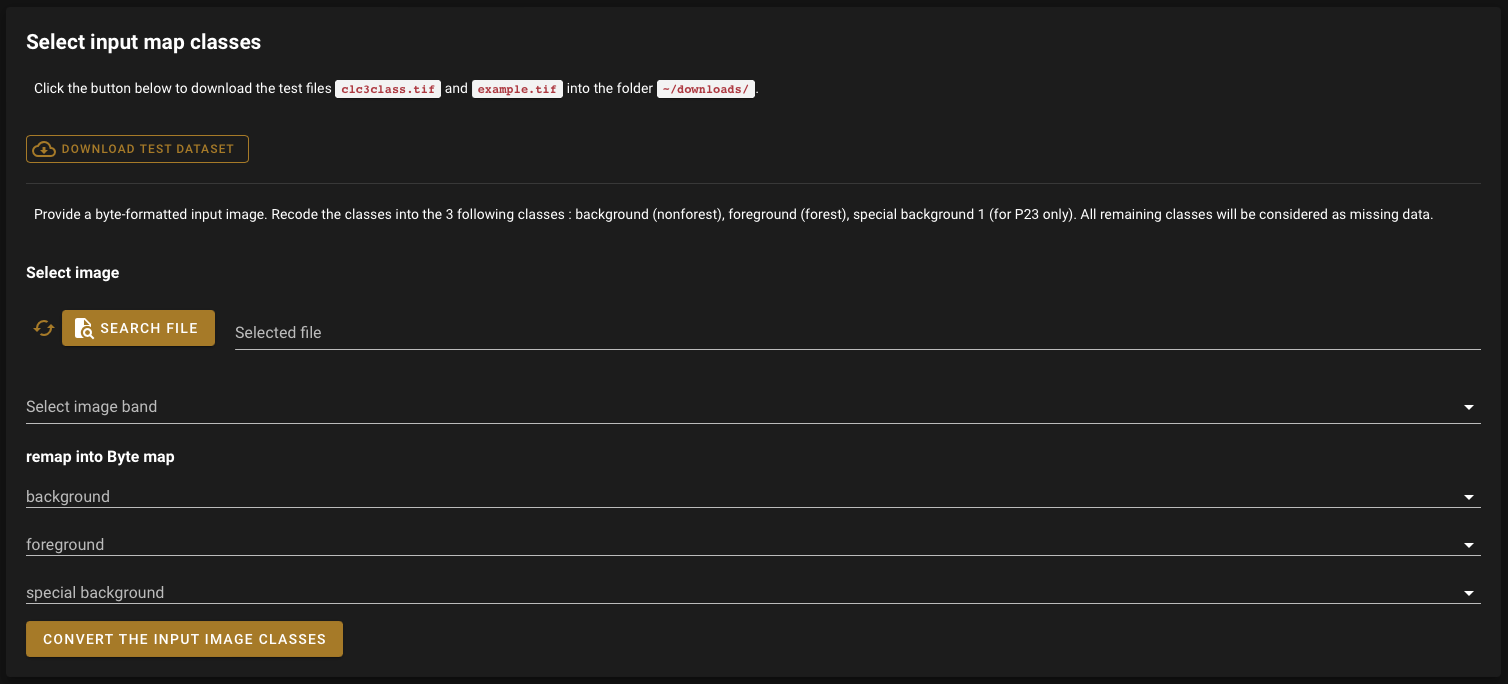
The dropdown menus will list the discrete values of your raster input image. Select each class in your image and place them in one of the following categories:
background
foreground
special background (for P23 only)
Every class that is not set to a reclassifying category will be considered as “missing data” (0 bytes).
Tip
For forest analysis, set Forest as foreground and all the other classes as background. If you specify a special background, it will be treated separately in the analysis (e.g. water, buildings).
Select the parameters#
You will need to select parameters for your computation:

Note
These parameters can be used to perform the default computation:
Window size: 27
Computation precision: Float (default)
Algorithm: FG-Density
Window size#
Set the square window size (in pixels). It should be an odd number in [3, 5, …501] with \(kdim\) being related to the observation scale by the following formula:
Also note that:
\(obs_scale\) in hectares
\(pixres\) in metres
\(kdim\) in pixels
Computation precision#
Set the precision used to compute your image. Float precision (default) will give more accurate results compared to rounded byte, but will also take more computing resources and disk space.
Algorithm#
The P223 module can run: FG-Density (P2), FG-Contagion (P22), or FG-Adjacency (P23).
P223 will provide a color-coded image showing [0,100]% for either FG-Density, FG-Contagion, or FG-Adjacency masked for the foreground cover. Use the alternative options to obtain the original spatcon output without normalization, masking or color-coding.
Tip
For original spatcon output ONLY: Missing values are coded as 0 (rounded byte), or -0.01 (float precision). For all output types, missing indicates that the input window contained only missing pixels.
Tip
For FG-Contagion and FG-Adjacency output ONLY: Missing also indicates that the input window contained no foreground pixels (there was no information about foreground edge).
For all output types, \(rounded byte = (float precision * 254) + 1\)
The options are displayed with the following names in the dropdown menu:
FG-Density (FG-masked and normalized)
FG-Contagion (FG-masked and normalized)
FG-Adjacency (FG-masked and normalized)
FG-Density (original spatcon output)
FG-Contagion (original spatcon output)
FG-Adjacency (original spatcon output)
FG-Shannon (original spatcon output)
FG-SumD (original spatcon output)
Run the analysis#
Once your parameters are set, you can launch the analysis. The blue rectangle will display information about the computation. Upon completion, it will turn green and display the Computation log.
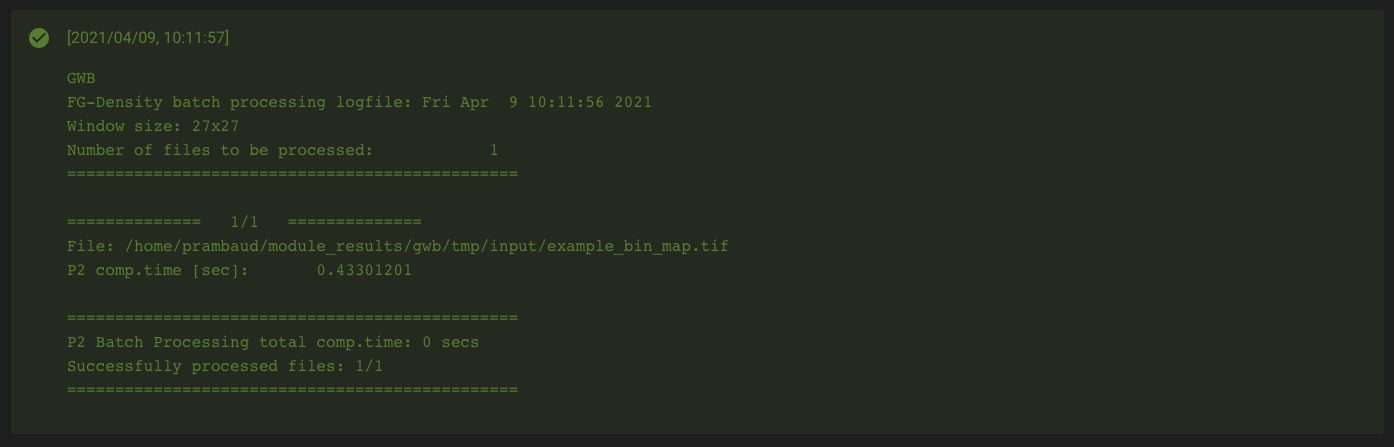
The resulting files are stored in the folder module_results/gwb/p223/. For example:
<raster_name>_bin_map.tif<raster_name>_bin_map_p<option>_<window>.tif<raster_name>_bin_map_p<option>_<window>.txt
Attention
If the rectangle turns red, carefully read the information in the log. For example, your current instance may be too small to handle the file you want to analyse. In this case, close the app, open a bigger instance and run your analysis again.
Here is the result of the computation using the P2 (Foreground-Density) option on the example.tif file.

Parcellation (PARC)#
This module will conduct the Parcellation analysis, providing a statistical summary file (.txt/.csv format) with details for each unique class found in the image, as well as the full image content: class value, total number of objects, total area and degree of parcellation.
Details on the methodology and input/output options can be found in the Parcellation product sheet.
Set up the input image#
Tip
You can use the default dataset to test the module. Select the Download test dataset button on the top of the second pane, which will add the following files to your downloads folder:
example.tif: 0 bytes - Missing, 1 byte - Background, 2 bytes - Foregroundclc3class.tif: 1 byte - Agriculture, 2 bytes - Natural, 3 bytes - Developed
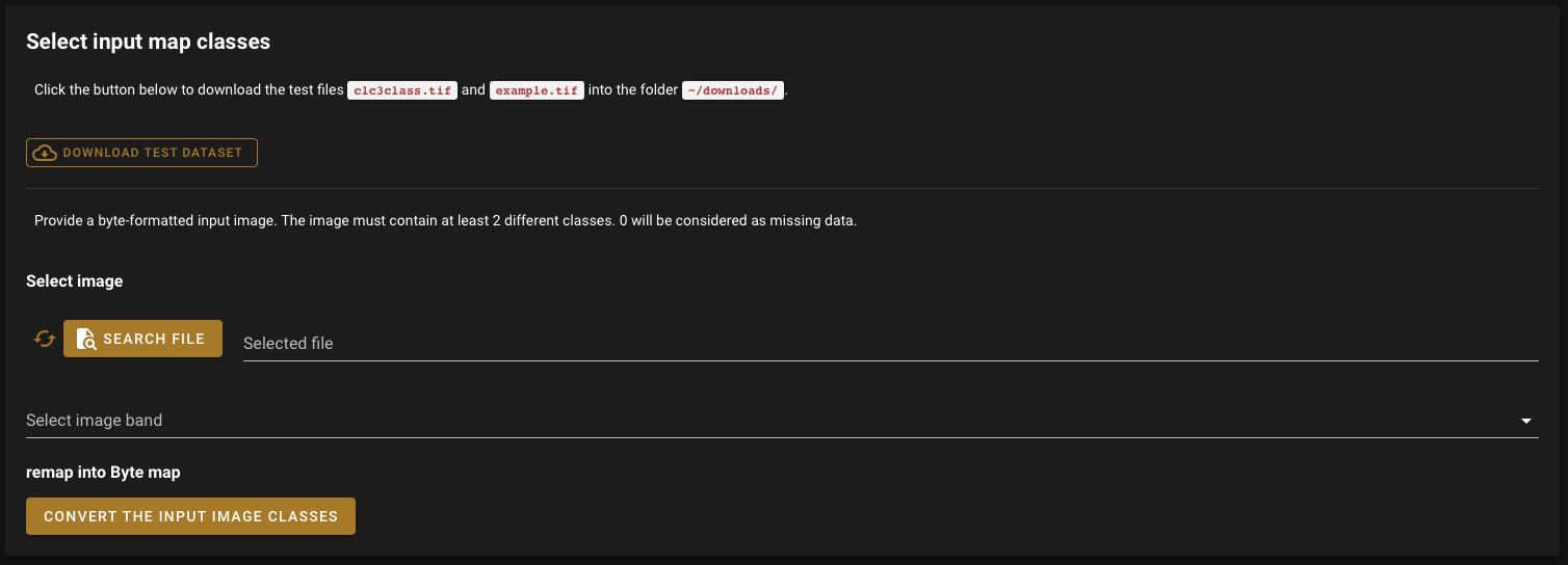
Once the files are downloaded, follow the normal process using the downloads/clc3classes.tif file (three classes).
The first step requires selecting your image in your SEPAL folders. The image must be a categorical .tif raster.
Attention
If the image is on your local computer and not in your SEPAL folders, see Exchange files with SEPAL.
Select the parameters#
You will need to select parameters for your computation:
Note
This parameter can be used to perform the default computation:
Foreground connectivity: 8
Foreground connectivity#
This sets the foreground connectivity of your analysis:
8 neighbours (default) will use every pixel in the vicinity (including diagonals)
4 neighbours will only use the vertical and horizontal one
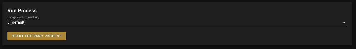
Run the analysis#
Once your parameters are all set, you can launch the analysis. The blue rectangle will display information about the computation. Upon completion, it will turn green and display the Computation log.

The resulting files are stored in the folder module_results/gwb/parc/. For example:
<raster_name>_bin_map.tif<raster_name>_bin_map_parc.csv<raster_name>_bin_map_parc.txt
Attention
If the rectangle turns red, carefully read the information in the log. For example, your current instance may be too small to handle the file you want to analyse. In this case, close the app, open a bigger instance and run your analysis again.
Here is the result of the computation using the default parameters on the clc3classes.tif file:
Class |
Value |
Count |
Area[pixels] |
APS |
AWAPS |
AWAPS/data |
DIVISION |
PARC[%] |
|---|---|---|---|---|---|---|---|---|
1 |
1 |
45 |
2.44893e+06 |
54420.7 |
2.07660e+06 |
1.27136e+06 |
0.152039 |
1.19374 |
2 |
2 |
164 |
5840.73 |
82557.6 |
19770.0 |
0.913812 |
17.7426 |
|
3 |
3 |
212 |
2798.07 |
19008.4 |
0.783919 |
11.0897 |
||
8-connected Parcels: |
421 |
4000000 |
9501.19 |
1310139.4 |
0.672465 |
8.07904 |
Restoration status summary (RSS)#
This module will conduct the Restoration status summary analysis, which will calculate key attributes of the current network status, composed of foreground (forest) patches, as well as provide the normalized degree of network coherence.
The results are tabular summary statistics.
Details on the methodology and input/output options can be found in the Restoration Planner product sheet.
Set up the input image#
Tip
You can use the default dataset to test the module. Select the Download test dataset button on the top of the second pane, which will add the following files to your downloads folder:
example.tif: 0 byte - Missing, 1 byte - Background, 2 bytes - Foregroundclc3class.tif: 1 byte - Agriculture, 2 bytes - Natural, 3 bytes - Developed
Once the files are downloaded, follow the normal process using the downloads/example.tif file (two classes).
The first step requires reclassifying your image. Using the Reclassifying pane, select the image in your SEPAL folders.
Attention
If the image is on your local computer and not in your SEPAL folders, see Exchange files with SEPAL.
The dropdown menus will list the discrete values of your raster input image. Select each class in your image and place them in one of the following categories:
background
foreground
Every class that is not set to a reclassifying category will be considered “missing data” (0 bytes).
Tip
For forest analysis, set Forest as foreground and all other classes as background.
Select the parameters#
You will need to select parameters for your computation:
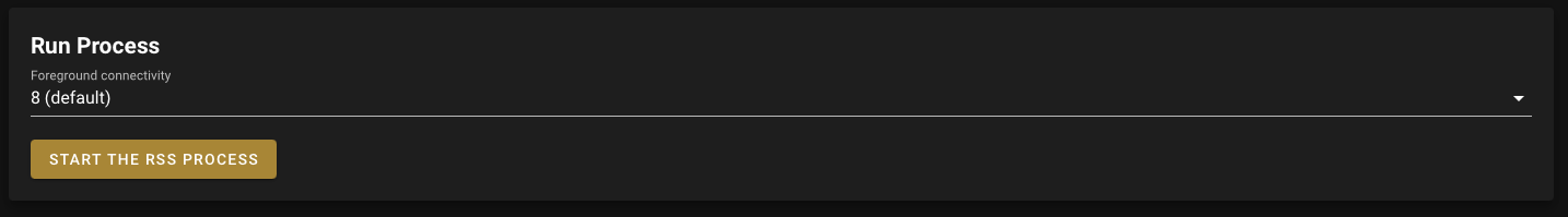
Note
These parameters can be used to perform the default computation:
Foreground connectivity: 8
Foreground connectivity#
This sets the foreground connectivity of your analysis:
8 neighbours (default) will use every pixel in the vicinity (including diagonals)
4 neighbours will only use the vertical and horizontal one
Run the analysis#
Once your parameters are set, you can launch the analysis. The blue rectangle will display information about the computation. Upon completion, it will turn green and display the computation log.
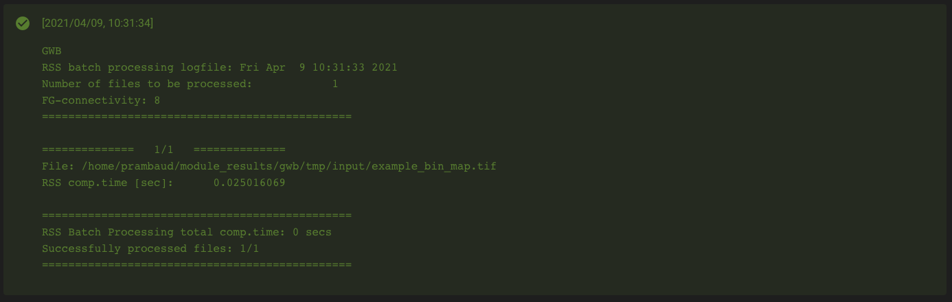
The resulting files are stored in the folder module_results/gwb/rss/. For example:
<raster_name>_bin_map.tifrss<connectivity>.txtrss<connectivity>.csv
Attention
If the rectangle turns red, carefully read the information in the log. For example, your current instance may be too small to handle the file you want to analyse. In this case, close the app, open a bigger instance and run your analysis again.
Here is the result of the computation using the default parameters on the example.tif file:
FNAME |
AREA |
RAC[%] |
NR_OBJ |
LARG_OBJ |
APS |
CNOA |
ECA |
COH[%] |
REST_POT[%] |
|---|---|---|---|---|---|---|---|---|---|
example_bin_map.tif |
428490.00 |
42.860572 |
2850 |
214811 |
150.34737 |
311712 |
221292.76 |
51.644789 |
48.355211 |
Simplified pattern analysis (SPA)#
This module will conduct the Simplified pattern analysis, which shapes and conducts a segmentation of foreground patches into two, three, five or six feature classes.
The results are spatially explicit maps and tabular summary statistics.
GWB_SPA is a simpler version of GWB_MSPA.
Details on the methodology and input/output options can be found in the Morphology product sheet.
Set up the input image#
Tip
You can use the default dataset to test the module. Select the Download test dataset button on the top of the second pane, which will add the following files to your downloads folder:
example.tif: 0 bytes - Missing, 1 byte - Background, 2 bytes - Foregroundclc3class.tif: 1 byte - Agriculture, 2 bytes - Natural, 3 bytes - Developed
Once the files are downloaded, follow the normal process using the downloads/example.tif file (two classes).
The first step requires reclassifying your image. Using the Reclassifying pane, select the image in your SEPAL folders.
Attention
If the image is on your local computer and not in your SEPAL folders, see Exchange files with SEPAL.
The dropdown menus will list the discrete values of your raster input image. Select each class in your image and place them in one of the following categories:
background
foreground
Every class that is not set to a reclassifying category will be considered “missing data” (0 bytes).
Tip
For forest analysis, set Forest as foreground and all other classes as background.
Select the parameters#
You will need to select parameters for your computation:
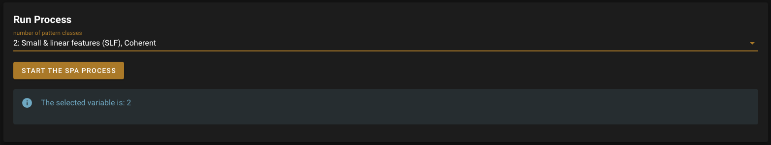
Note
This parameter can be used to perform the default computation:
number of pattern classes: 2: Small & linear features (SLF), Coherent
Number of pattern classes#
Set the number of pattern classes you want to compute:
2: Contiguous, Small & linear features (SLF)
3: Core, Core-Openings, Margin
5: Core, Core-Openings, Edge, Perforation, Margin
6: Core, Core-Openings, Edge, Perforation, Islet, Margin
Run the analysis#
Once your parameters are set, you can launch the analysis. The blue rectangle will display information about the computation. Upon completion, it will turn green and display the Computation log.
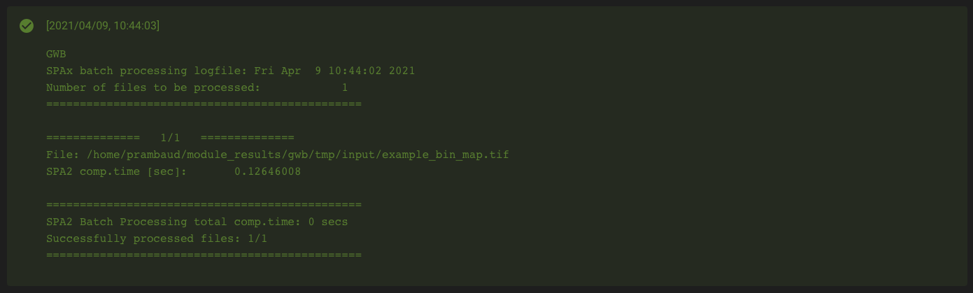
The resulting files are stored in the folder module_results/gwb/spa/. For example:
<raster_name>_bin_map.tif<raster_name>_bin_map_spa<number of classes>.tif<raster_name>_bin_map_spa<number of classes>.txt
Attention
If the rectangle turns red, carefully read the information in the log. For example, your current instance may be too small to handle the file you want to analyse. In this case, close the app, open a bigger instance and run your analysis again.
Here is the result of the computation using SPA2 (two classes) on the example.tif file:

References#
GuidosToolbox Workbench: Spatial analysis of raster maps for ecological applications