

Soil moisture mapping#
Map surface soil moisture based on Copernicus Sentinel-1 intensity data
Open SEPAL#
Tool for mapping surface soil moisture based on Copernicus Sentinel-1 intensity data
Open SEPAL and log in.
To open SEPAL in your browser, go to https://sepal.io/.
Connect SEPAL to your Google account.
Make sure SEPAL is connected to your Google account (see Use GEE with SEPAL).
Upload your area of interest (AOI) shapefile as a Google Earth Engine (GEE) asset.
Instructions for uploading a shapefile as an asset can be found here: https://developers.google.com/earth-engine/importing
Start an
m4instance in the terminal.
Process Sentinel-1 time series data to generate maps of soil moisture#
Open and launch the Soil moisture mapping application.
To access the module, select the Apps tab in SEPAL. Use the search box and enter “SOIL MOISTURE MAPPING”, or find it manually.
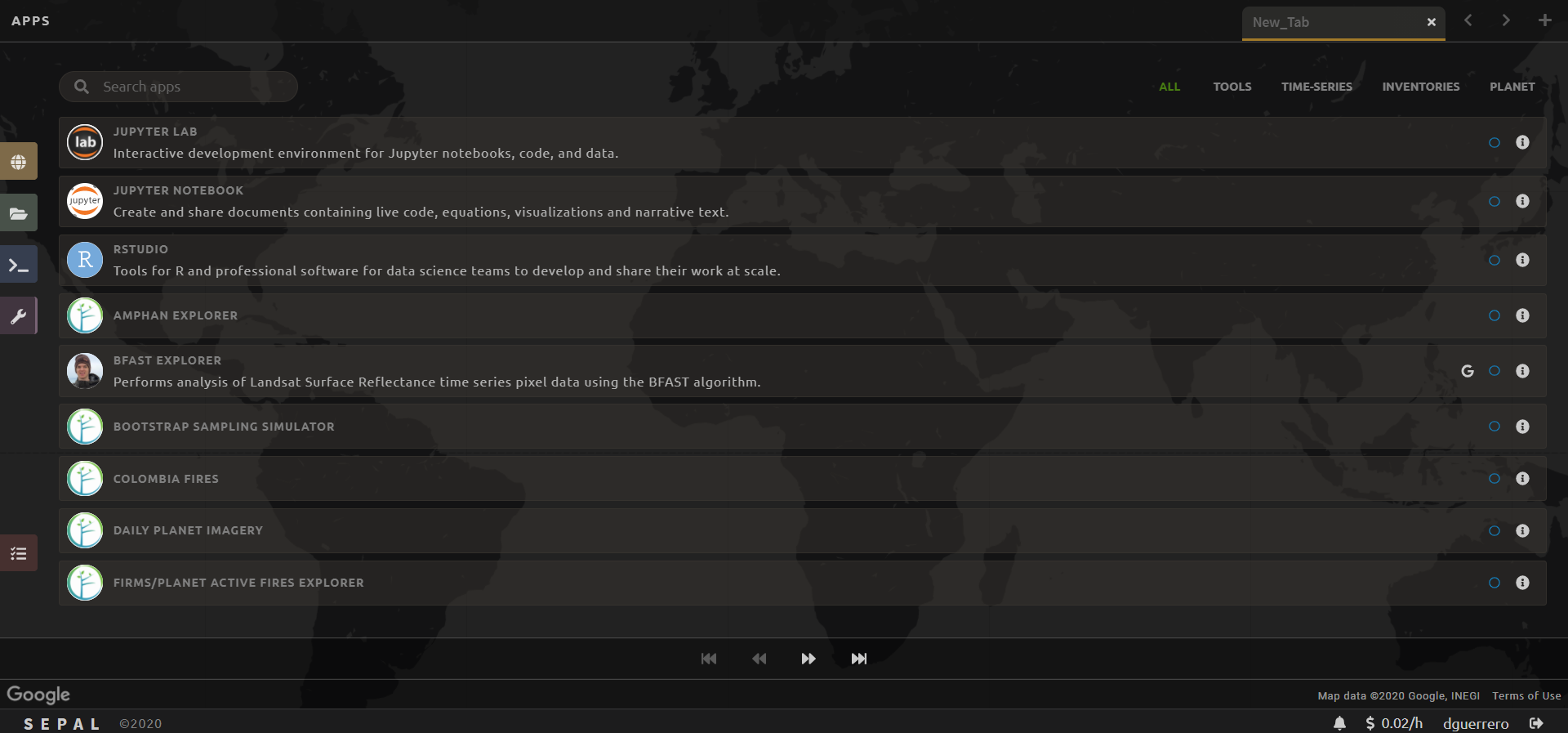
The application will be launched and displayed over a new tab in the SEPAL pane.
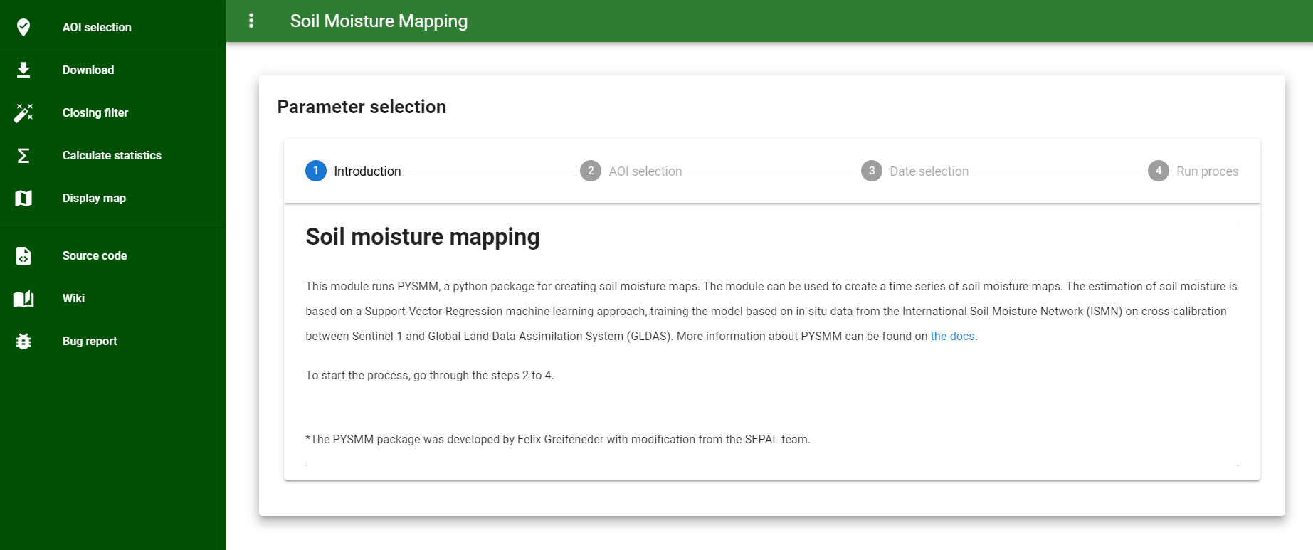
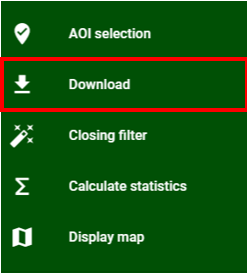
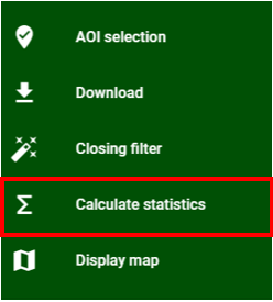
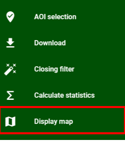
The module has five main steps that can be selected in the left pane: AOI selection, download, closing filter, calculate statistics, and display map.
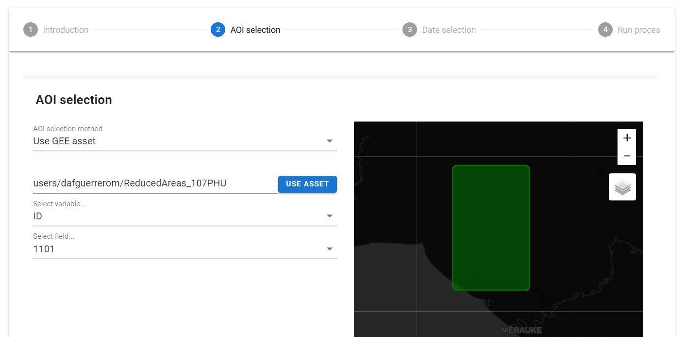
Select the AOI selection step and follow the next four sub-steps.
In the AOI selection step, choose Use GEE asset. Paste your GEE asset ID into the box and select the “Use asset” button to select your AOI.
Two new selection dropdown menus will appear. Choose your variable and field, then wait until the polygon is loaded onto the map.
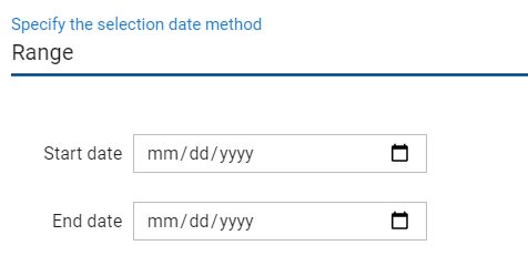
Select the date range of the data that you want to process through GEE. There are three options:
Single date: Process one soil moisture closest to the date selected.
Range: Process all Sentinel-1 data to create a time series of soil moisture maps for the date range selected.
All-time series: Process all available Sentinel-1 data since the launch of the satellite in 2015 to create a time series of soil moisture maps.
Initiate soil moisture processing.
After the filters are selected, go to the Run process tab.
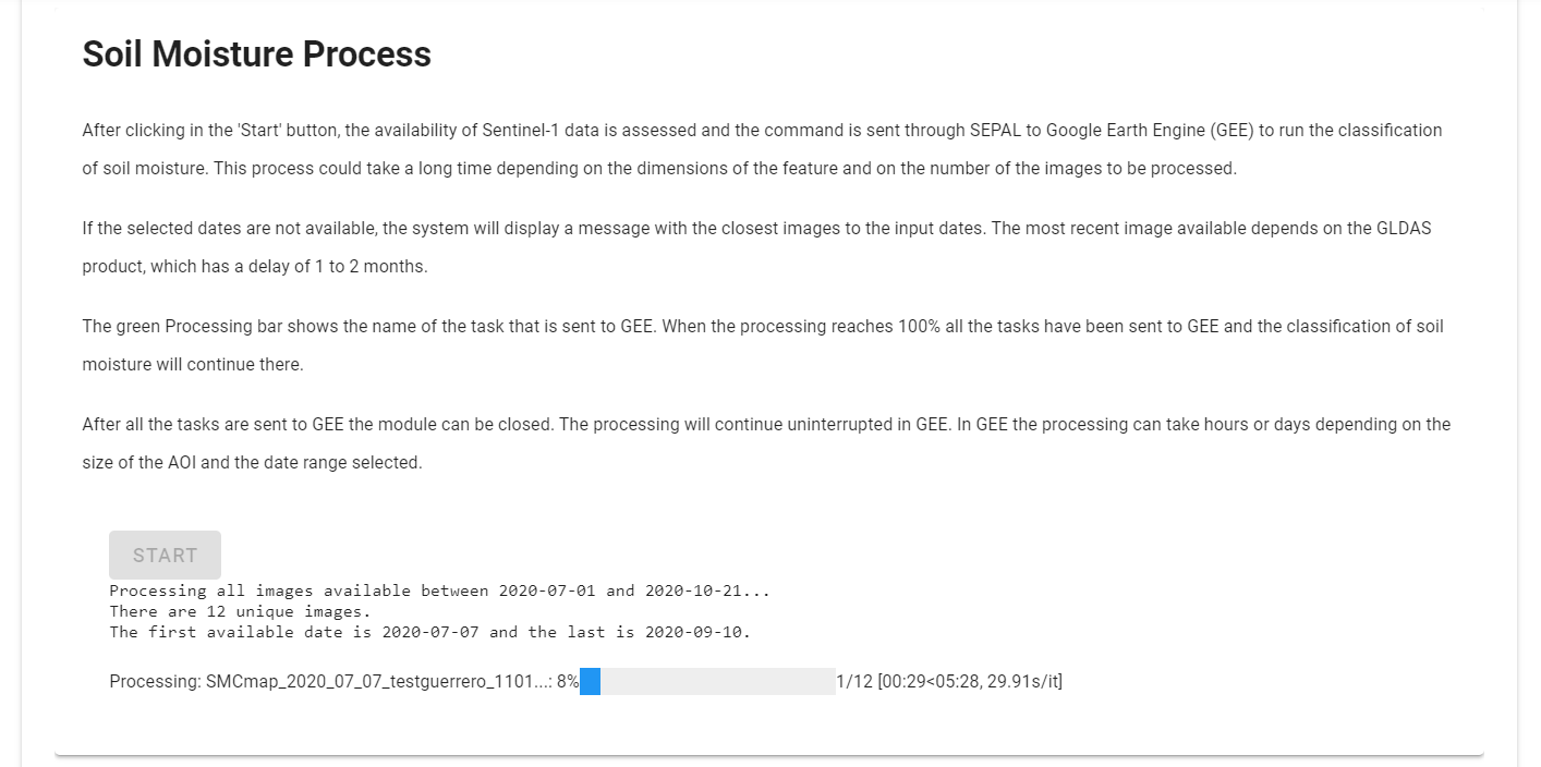
Once the Start button has been selected, the availability of Sentinel-1 data is assessed and the command is sent to GEE to run the classification of soil moisture.
This process could take a long time depending on the dimensions of the feature and the number of images to be processed.
If the selected dates are not available, the system will display a message with the closest images to the input dates.
The most recent image available depends on the Global Land Data Assimilation System (GLDAS) product, which has a delay of one to two months.
The green Processing bar shows the name of the task that is sent to GEE. When the processing reaches 100 percent, all tasks have been sent to GEE and the classification of soil moisture will continue there.
After all tasks are sent to GEE, the module can be closed. The processing will continue uninterrupted in GEE, where it can take hours or days depending on the size of the AOI and the date range selected.
Check the progress of the soil moisture processing GEE.
Go to the GEE code editor to check on the status of each task.
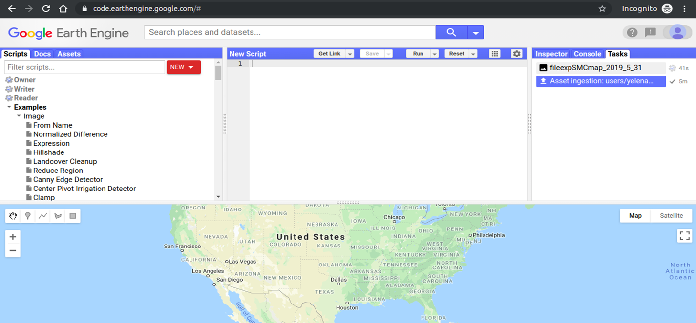
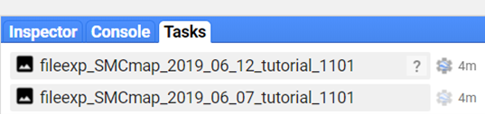
Select the Tasks tab in the section on the right. You should see the process running with the spinning gear.
When the download completes, you will see a blue checkmark. Check periodically on your download to make sure all specified dates are being downloaded.
Download soil moisture maps from GEE to SEPAL#
Check if the processing is complete in GEE.
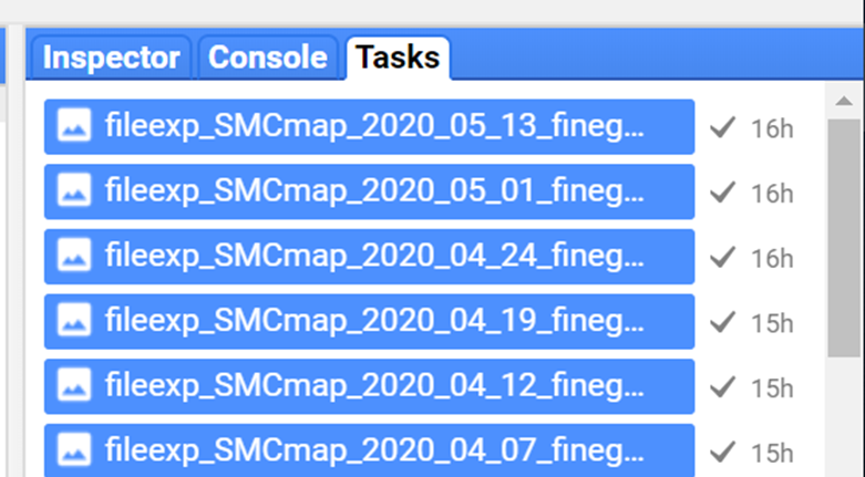
Check on the status of each task in the GEE code editor. Select the Tasks tab in the section on the right. You should see blue checkmarks next to all tasks.
Soil moisture maps for each date have been downloaded to your Google Drive. The next step will automatically move those images from your Google account to your SEPAL account.
You can start downloading the images while they are being processed in GEE, but we recommend waiting until all or part of the images have been processed in GEE.
Use the download step.
In the left pane, select the Download button.
Select the download task file.
The file structure for downloading and managing soil moisture data follows this structure:
home/username/pysmm_downloads/0_raw/asset_name/row_nameAll downloads can always be found in the pysmm_downloads folder.
Each time a different asset is used to derive soil moisture, a new folder for the asset will be created.
For each polygon that is used from the asset, selected by specifying the column and row field names, a unique folder with the row field name will contain the task download file.
The task download file can be found in the folder
home/user/ pysmm_downloads/0_raw/assetname/rowname/The task download file naming convention is: task_datedownloadinitiated_code.txt
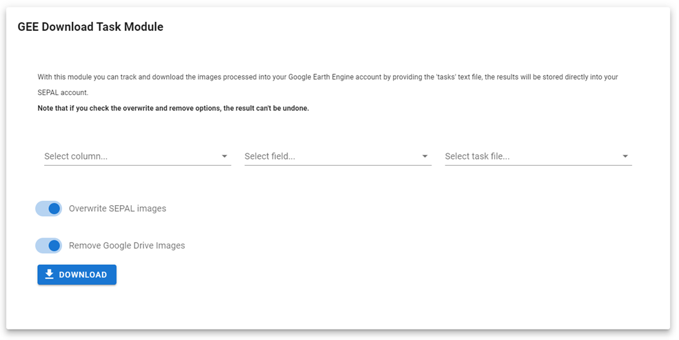
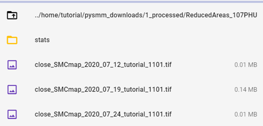
Use the three dropdown lists to choose the desired task text file by selecting the folder names.
There are options to overwrite duplicates already downloaded into SEPAL and remove downloaded images from Google Drive. Once the images are removed from Google Drive, the task download file will no longer function because those images will not be stored in Google Drive.
Overwrite SEPAL images: In case you previously have downloaded an image in the same path folder, the module will overwrite the images with the same name.
Remove Google Drive images: Mark this option if you want to download the images to your SEPAL account and delete the files from your Google Drive account.
Select the DOWNLOAD button to download the soil moisture maps from your Google Drive account to SEPAL.
The images will download separately; leave the application open while the download is running.
After the data download is complete, you can use tools available in SEPAL to process and analyse the soil moisture maps.
Post-process and analyse soil moisture time series data#
After the download is complete, apply a robust methodology for image filtering to fill no-data gaps and assess trends in the time series of soil moisture maps.
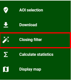
Select the Closing filter step.
In the left pane, select the Closing filter tab.
Run the post-processing section of the module.
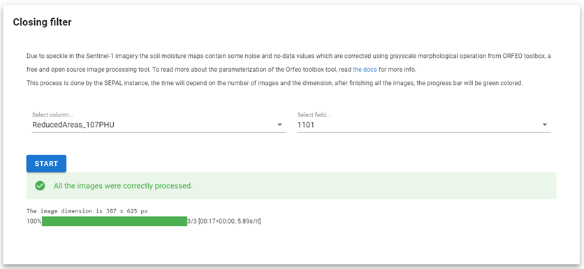
Navigate to the folder where the images are stored. This module will process a folder with many images, going through each of the images. Therefore, the input should be the folder in which the raw images are stored. The module will automatically display two selection menus; select the desired options.
The raw imagery is stored in the same folder that the task download file is located.
Select the START button to run a data-filling algorithm on each of the soil moisture maps.
Due to speckle in Sentinel-1 imagery, soil moisture maps contain some noise and no-data values which are corrected to some extent using grayscale morphological operation from ORFEO toolbox, a free and open-source image processing tool (see https://www.orfeo-toolbox.org/CookBook/Applications/app_GrayScaleMorphologicalOperation.html.
This process is done by the SEPAL instance; the time will depend on the number of images and dimensions. After finishing all images, the Progress bar will turn green.
Run the Statistics post-process.
In the left pane, select the Calculate statistics tab.
After the data is filtered, a time series analysis of the soil moisture maps can be performed. Several statistics can be applied whether to the entire time series or to a specified range; statistics as median, mean, standard deviation, or linear trend (slope of the line) are available to process the selected data.
This module uses the Stack composed python module, which computes a specific statistic for all valid pixel values across the time series using a parallel process.
Select column and field to process all images inside that folder.
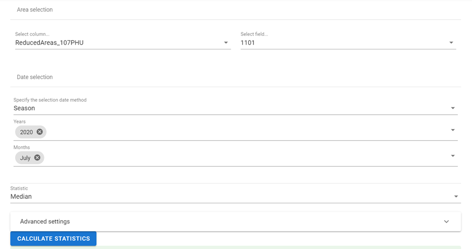
There are three options for analysing the data for different time frames.
All-time series: Run the analysis for all images in the folder.
Range: Run the analysis for all images within the selected time frame.
Season: Define a season by selecting months; the analysis is run for only the months selected within the years selected (e.g. if January, February, and 2016, 2017, 2018 are selected, then the analysis would run for January 2016, January 2017, January 2018, February 2016, February 2017, and February 2018). You can also select only one year or month, so it will process all the years/months in the selection.
There are different options for the statistics that can be calculated. The options include:
Median
Mean
Gmean: geometric mean
Max
Min
Std: standard deviation
Valid pixels
Linear trend
The Valid pixels option will create a new image representing only the count of the valid pixels from the stack.
The Median, Mean, Geometric Mean, Max, Min, Standard Deviation and Valid pixels are statistics that do not require much computing requirements, so the time to perform those tasks is relatively quick, depending on the extent of the image.
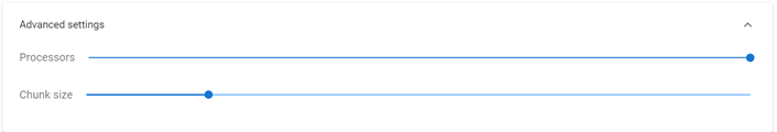
The Advanced settings are intended to be used to improve the time and manage system resources. Normally, this is automatically optimized, but can be modified by the user. This setting controls the number of processors you use for parallel processing, allowing you to optimize the time by processing a huge image by using several processors at the same time (by default, all available processors will be used; note that the more CPUs available in the selected instance in the terminal, the faster the processing will be).
Processors: By default, the module will display the number of processors that are active in the current instance session and will perform the stack composed with all of them; however, in order to test the best benchmark to the specific stack, this number could be changed within the Advanced settings tab.
Chunks: The number in the chunk specifies the shape of the array that will be processed in parallel over the different processors (i.e. if 180 is the specified number of chunks, then the stack-composed module will divide the input image into several small square pieces of 180 pixels with its shape). For more information about how to select the best chunk shape, follow the documentation.
Once the settings are specified, select the Calculate statistics button.
After selecting the temporal range to run the analysis and parameters to calculate, the images that are processed are listed along with the date of the imagery.
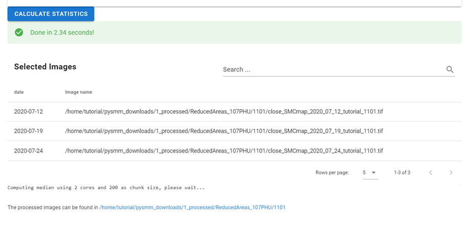
The processed images can be found in the folder: home/user/pysmm_downloads/1_processed/assetname/rowname/stats
Visualizing imagery#
In the left pane, select the Display map tab.
The Map visualization tab will allow you to display any mono-band image in your SEPAL account (not only the downloaded data).
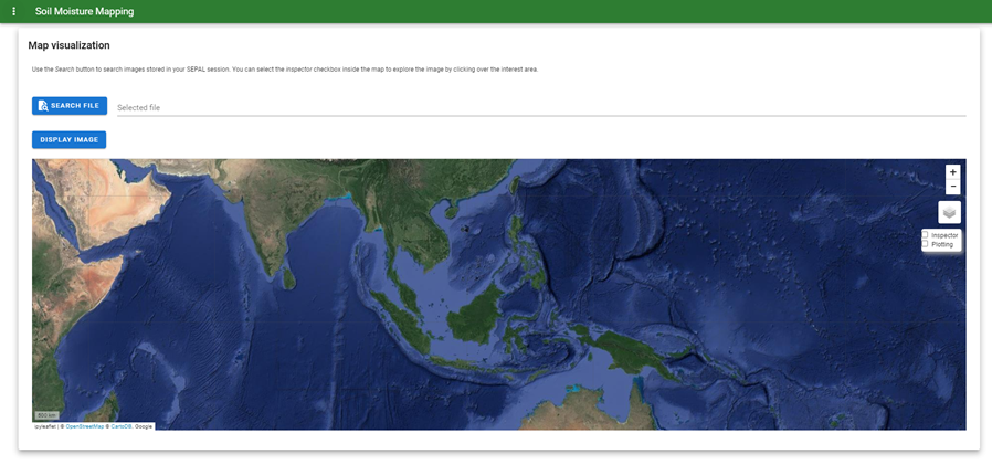
Select the Search file button and navigate over the dropdown list to search for the desired image. Select the Display image button.
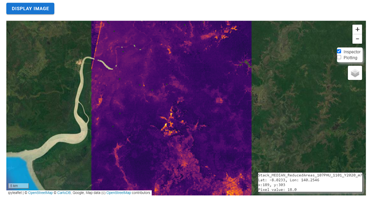
Wait until the image is rendered on the map and explore the general output.
Mark the Inspector checkbox and click over any coordinate inside the image to explore the pixel values; you will see an output box in the lower-right corner with the data.
Open-source data from Sentinel-1 operates using C-band synthetic aperture radar imaging. C-band type has a wavelength of 3.8–7.5 cm, and thus has limited penetration into dense forest canopies. Therefore, forested areas should be excluded from the analysis. L-band data should be used instead of such areas.
It is recommended that densely vegetated areas are excluded from analysis due to the limitation of C-band radar to penetrate dense canopy cover. Use a forest map to exclude dense forest areas from the analysis.