Satellite Monitoring for Forest Management – Biomass Tool for ALOS tool (SMFM BIOTA)

The Biomass Tool for ALOS (BIOTA tool) is part of the World Bank’s project, Satellite Monitoring for Forest Management (SMFM) project. It was developed by LTS International and the University of Edinburgh with an integration in the SEPAL platform developed by the SEPAL developer team.

The tool relies on the use of JAXA’s ALOS PALSAR L-band mosaics, allowing users to produce outputs of:

• calibrated Gamma0 backscatter

• forest cover

• above-ground biomass (AGB)

• ABG change

• classified forest change types (deforestation, degradation, etc.)

In this exercise, you will learn how to use the BIOTA tool to calculate AGB in dry forests and savannahs, as well as change maps.

Note

Objectives:

• Generate maps of AGB, Gamma0 backscatter, forest cover, AGB change, deforestation risk, and change type.

Attention

Prerequisites:

• SEPAL account

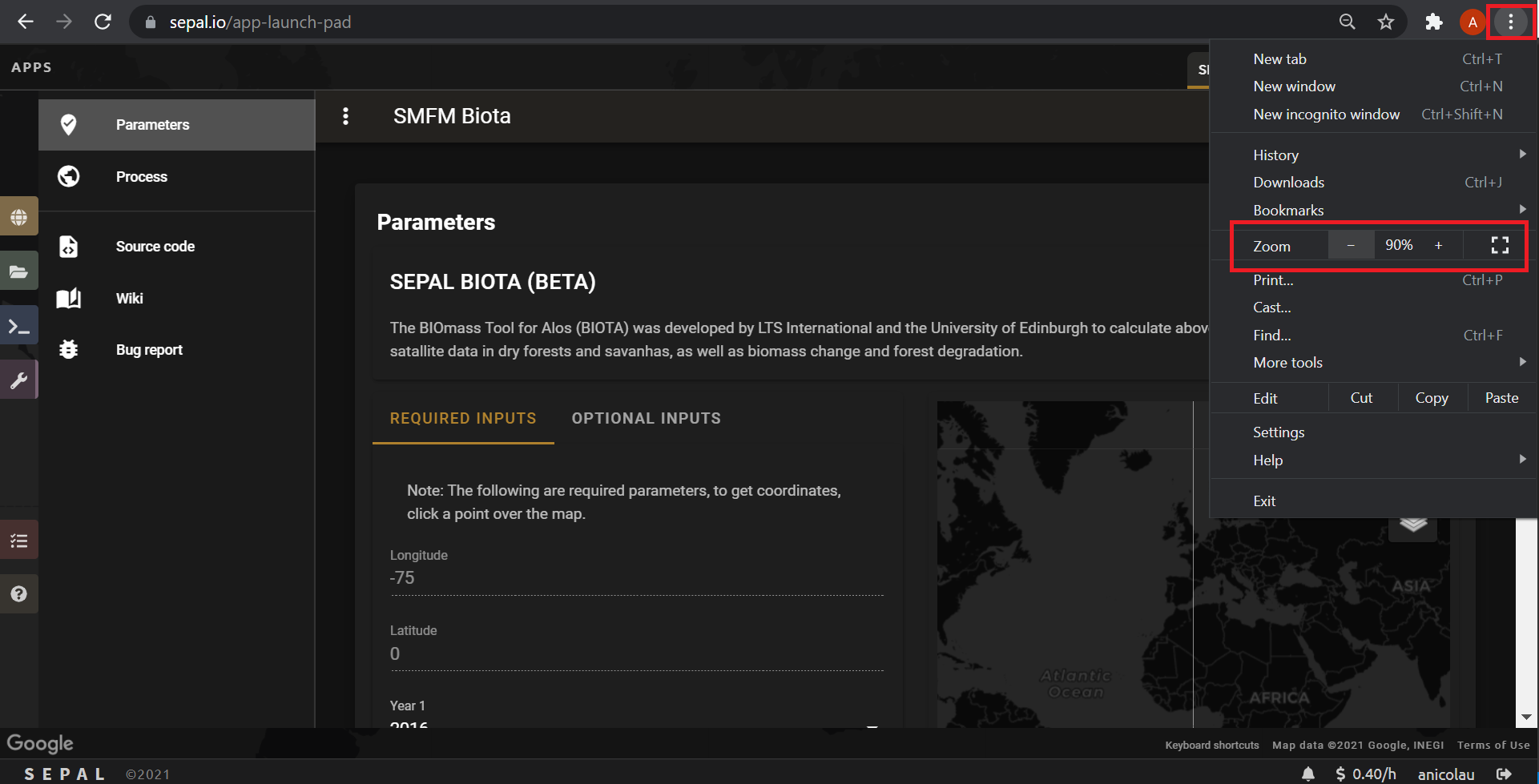
Navigate to the Apps menu by selecting the wrench icon and entering SMFM into the search field. Then, select SMFM Biota.

Note

Sometimes the tool takes a few minutes to load. Wait until you see the tool’s interface. In case the tool fails to load properly (see figure below), close the tab and repeat the aforementioned steps. If this does not work, reload SEPAL.

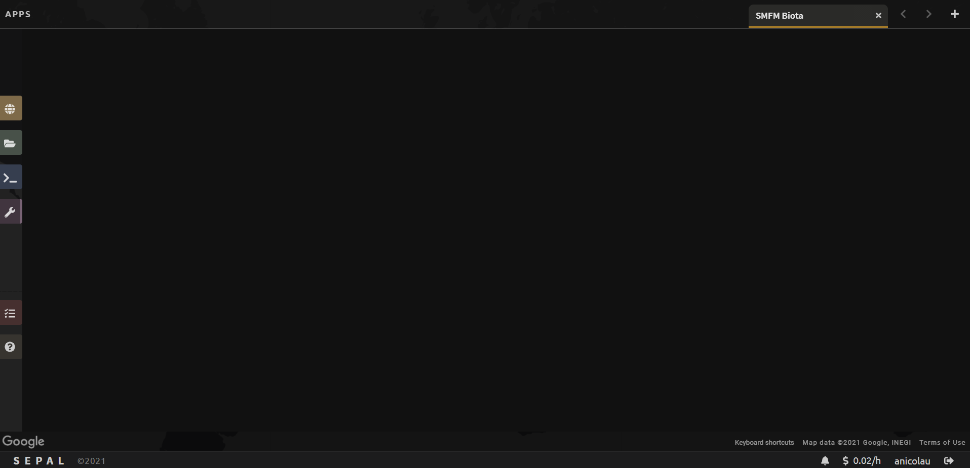
If none of these steps work, you might need to start another instance. Please see Introduction to SEPAL for steps on how to use the terminal to start a higher instance (an m4 instance should be enough). (You should see an interface like the one in the following figure.)

Tip

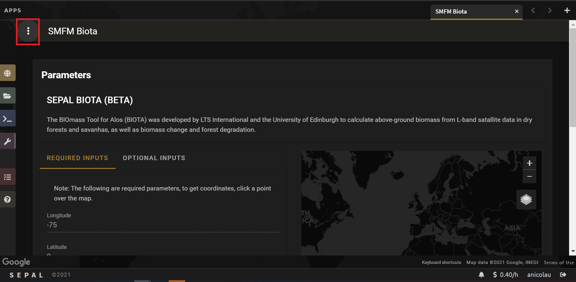
Depending on your computer screen size, the left column may appear on top of the content, as seen in the following figure.

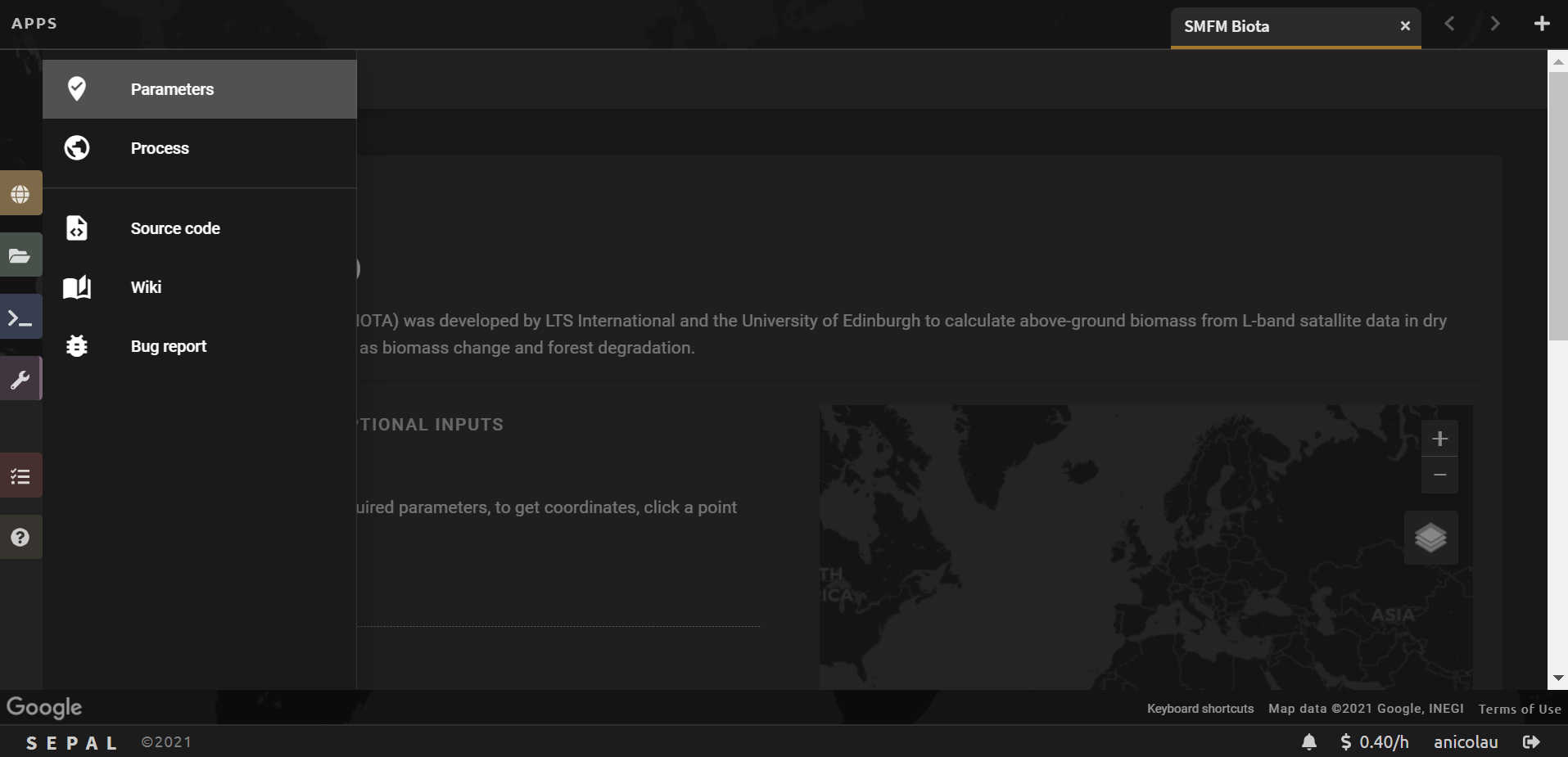
If this is the case, you can either:

• Adjust your browser zoom level, or

• Keep the zoom level, but click outside of the column to hide it. To open it again, you will need to select the three dots located in the upper-right.

Downloading ALOS mosaics

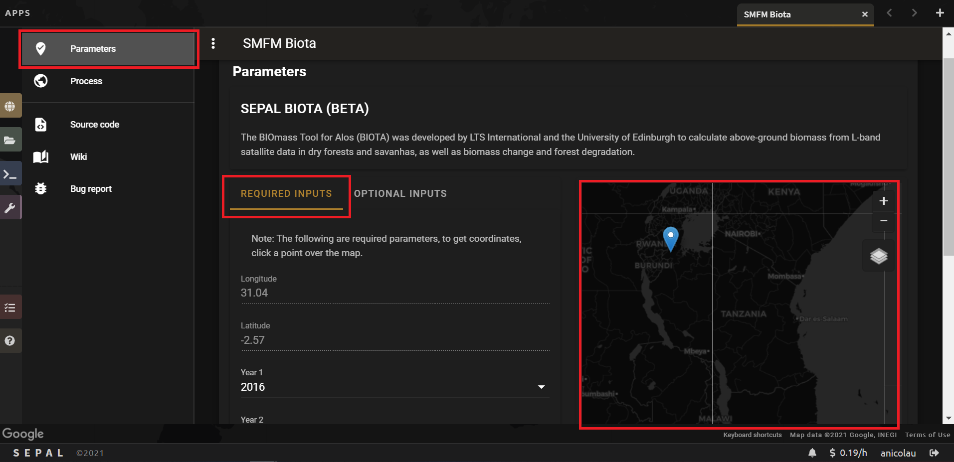
The first step is to select the parameters for accessing data from ALOS (JAXA). The data is delivered in SEPAL as either 1 x 1 degree tiles or 5 x 5 degree collections of tiles.

Under Required inputs, define the latitude and longitude coordinates by clicking on your point of interest on the map that is shown on the right (this will be the upper-left coordinate of the tiles). The default values are -75 degrees for longitude and 0 degrees for latitude. For this exercise, we will demonstrate the steps for a point between the Moyowosi Game Reserve and the Kigosi Game Reserve, next to the border of the Getta and Kigoma regions in Tanzania (latitude -2.54, longitude 31.04).

Note

The BIOTA tool was designed for woodlands and dry forests, as it uses a generic equation to calibrate Gamma0 backscatter to forest AGB developed using forest plot data from Malawi, Mozambique and Tanzania in southern Africa. For global applicability, the tool supports the calibration of country-specific backscatter–AGB relationships through determined parameters, which will be explained later in this page of the documentation.

Next, we define the two years of interest. For this exercise, we will leave the default values (2016 for Year 1 and 2017 for Year 2; Year 2 is used for calculating changes).

The tool gives you the option to choose a size of either a 1 x 1 degree tile or a 5 x 5 degree tile. We will select the 1 x 1 tile size for time purposes.

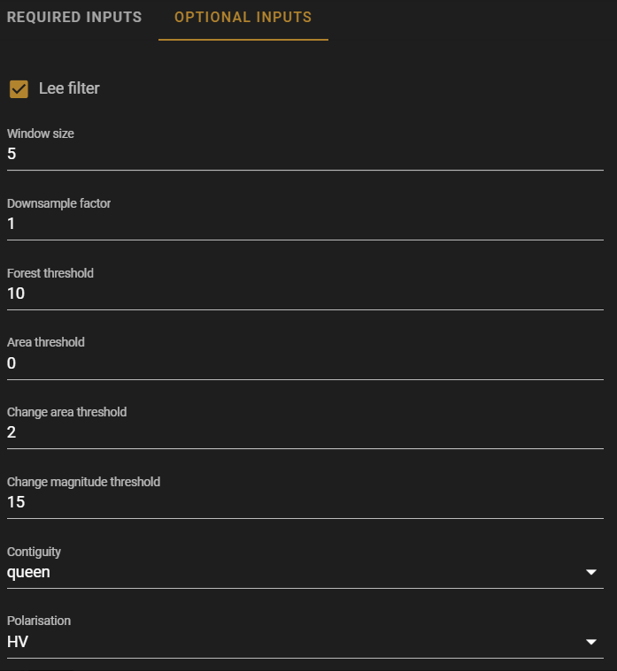
Before selecting Download images, we will look into the Optional inputs tab.

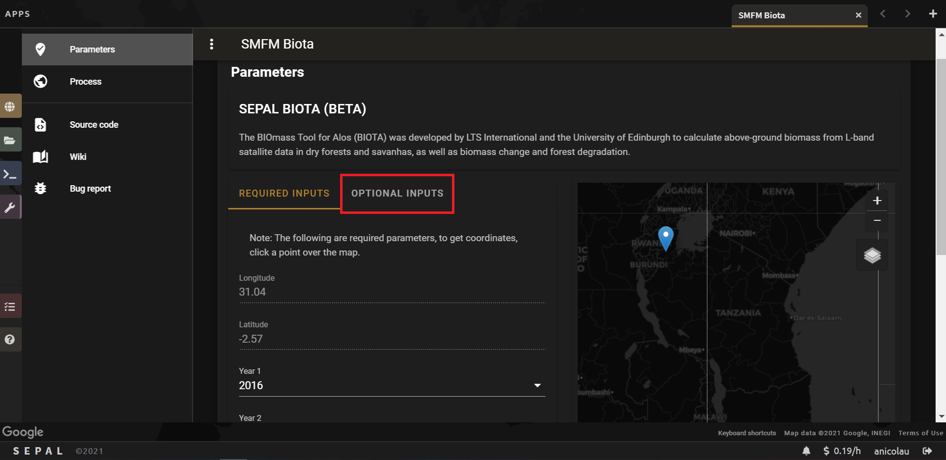
Different parameters can be changed here. These include the parameters that should be calibrated according to your AOI and specific forest characteristics. Default values are specific to southern African forests.

Parameter	Role
Lee filter	Applies a Lee filter to the data. This reduces inherent speckle noise in SAR imagery. Uncheck if you do not want the filter applied.
Window size	Lee filter window size. Defaults to 5 x 5 pixels.
Downsample factor	Applies downsampling to inputs by specifying an integer factor to downsample by. Defaults to 1 (i.e. no downsampling).
Forest threshold	A forest AGB threshold (in tonnes per hectare) to separate forest from non-forest (specific to your location). Defaults to 10 tC/ha.
Area threshold	A minimum area threshold (in hectares) to be counted as forest (e.g. a forest patch must be greater than 1 ha in size). Defaults to 0 ha.
Change area threshold	A threshold for a minimum change in forest area required to be flagged as a change. Defaults to 2 ha. This is for users who aim to produce change maps.
Change magnitude threshold	The minimum absolute change in biomass (in tonnes per hectare) to be flagged as a change. Defaults to 15 tC/ha. This is for users who aim to produce change maps.
Contiguity	The criterion of contiguity between two spatial units. The rook criterion defines neighbors by the existence of a common edge between two spatial units. The queen criterion is somewhat more encompassing and defines neighbours as spatial units sharing a common edge or a common vertex.
Polarization	Which SAR polarization to use. Defaults to HV.

We will leave the parameters with default values.

Now, go back to the Required inputs tab and select Download Images at the bottom. This will download all ALOS data tiles into your SEPAL account.

Note

Depending on your point coordinates, it may take a significant amount of time before your data finish downloading. For the point in Tanzania, it should take about five minutes.

You can see the status of the downloads at the bottom of the page.

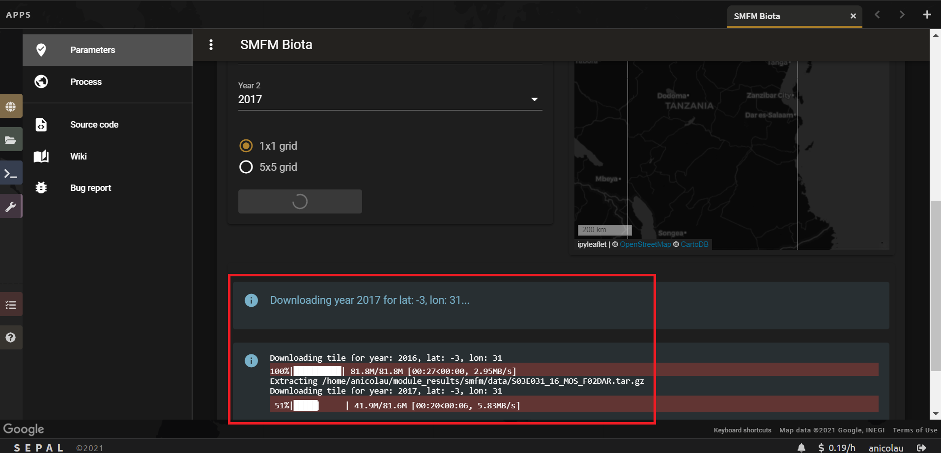
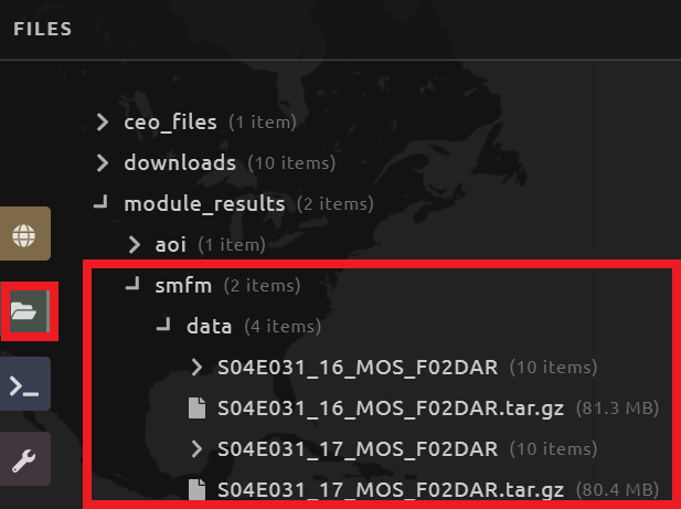
Once the downloads are finalized for both years, you are able to see the downloaded files under SEPAL Files. Go to module_results > smfm > data.

Here is a demonstration of the above steps:

Processing the data and producing outputs

Now that the download has finished, we can process the data to produce the desired outputs.

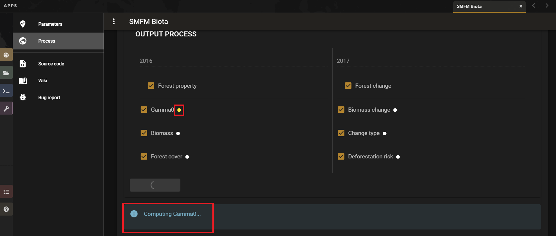
Select the Process tab on the left side.

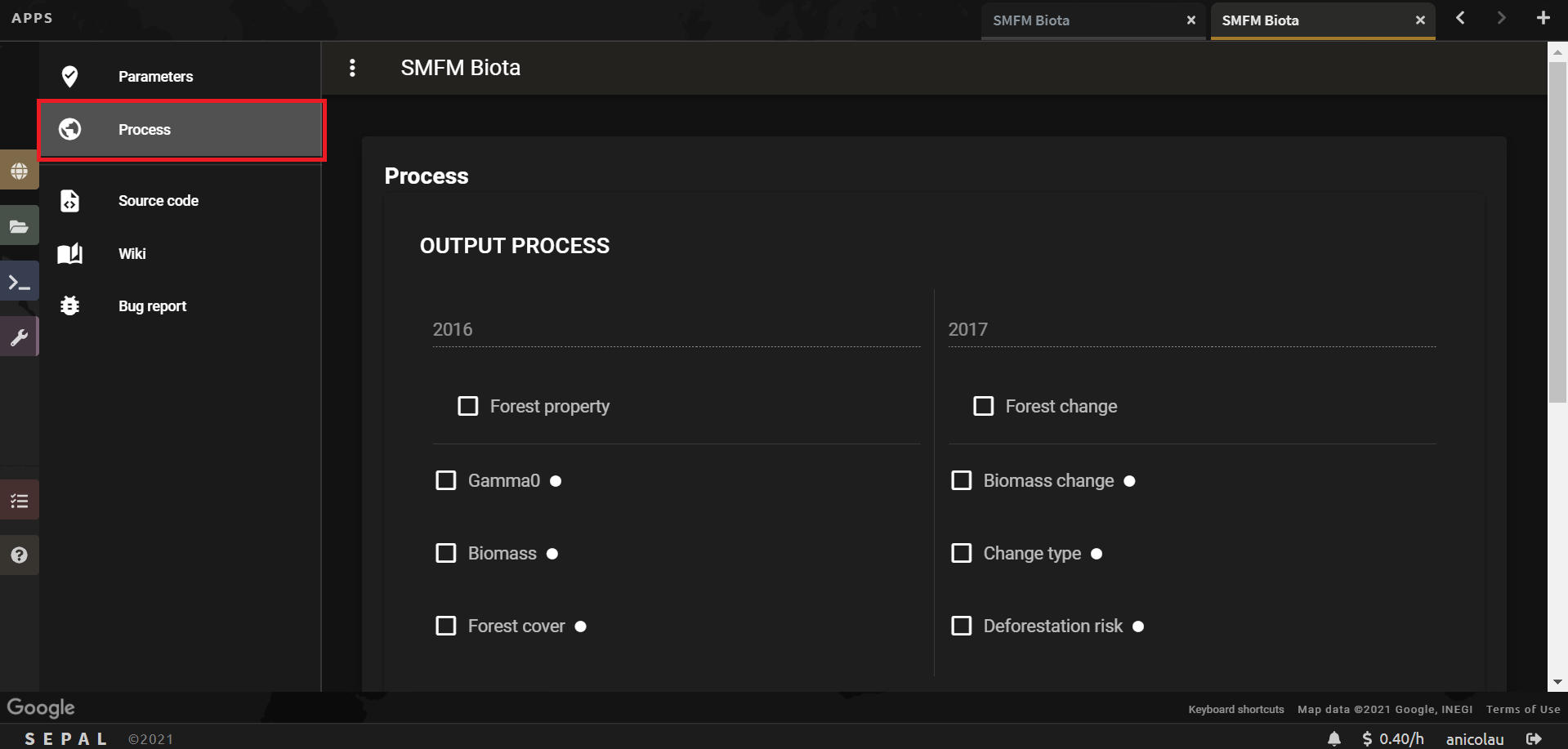
For Year 1, we will choose Forest property, which will automatically check all outputs available (“Gamma0”, “Biomass”, “Forest Cover”). For Year 2, we will choose Forest change (changes between 2016 and 2017), which will also select all available outputs (“Biomass change”, “Change type”, “Deforestation risk”). These will be explained later.

Select Get outputs to start the processes.

Note

Depending on your point coordinates, it may take a significant amount of time before your data finish downloading (for the point in Tanzania, it should take approximately two minutes).

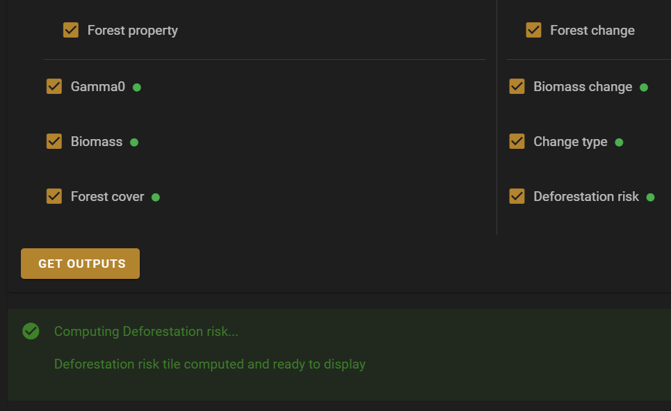
Similarly to before, the tool will show the process status at the bottom. You will also note a change of color from white to yellow next to each output (white = not started, yellow = processing, green = finalized).

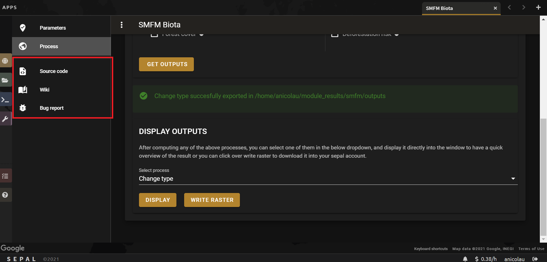
Once complete, you will see a message similar to the one below, and all outputs will have a green “light”.

Here is a demonstration of the above steps:

Displaying your outputs

With the outputs processed, we can now visualize the results.

In the same window, under Display outputs, you can choose the process to display by selecting the dropdown ‘Select process’ option.

Select Biomass. Then, press Display. You will see the map appear on your screen (see figure below).

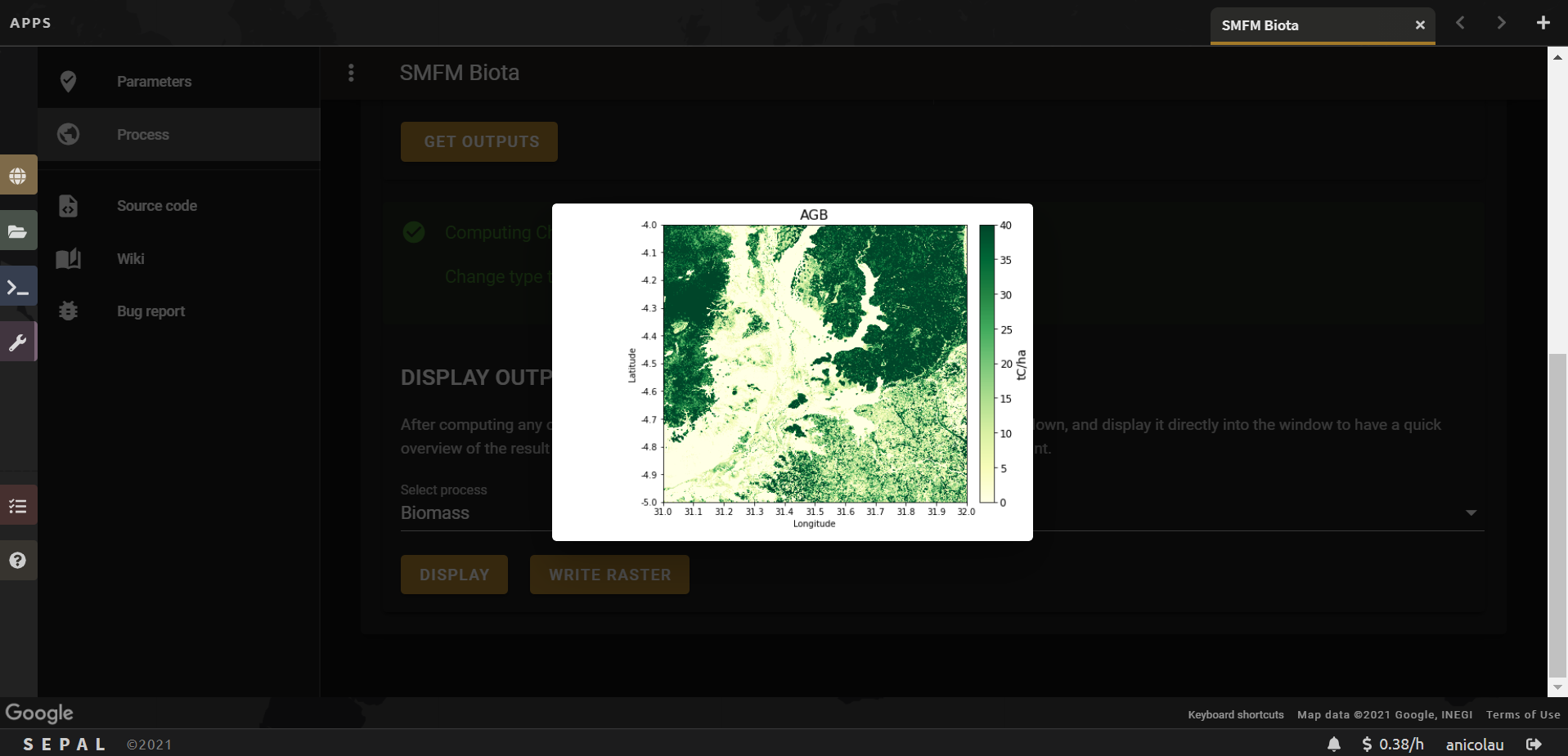
This is showing AGB in tonnes per hectare (tC/ha) for the 1 x 1 degree tile in Tanzania. To go back to the interface and select the other outputs, you can click anywhere on the screen outside of the map and do the same for the other results.

If you followed these exact steps, your outputs should look similar to the ones in the figure below.

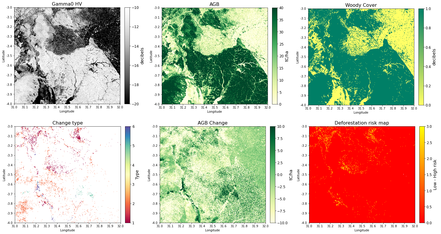
A summary of each output is described in the table below.

Output	Description
Gamma0	Gamma0 backscatter in decibels for the polarization specified
Biomass	Biomass in tonnes per hectare
Forest/woody cover	Binary classification of forested (1) and non-forested (0) areas
Change type	Change described in seven different types (specified below)
Biomass change	Change in biomass in tonnes per hectare
Deforestation risk	Risk of deforestation from Low (1) to High (3)

There are seven change types described in the BIOTA tool, each of which is defined as a number (0 to 6) and color-coded on the map. Change types include:

Change class	Pixel value	Description
Deforestation	1	A loss of AGB that crosses the forest_threshold.
Degradation	2	A loss of AGB in a location above the forest_threshold in both images.
Minor loss	3	A loss of AGB that does not cross the change_area_threshold or change_magnitude_threshold.
Minor gain	4	A gain of AGB that does not cross the change_area_threshold or change_magnitude_threshold.
Growth	5	A gain of AGB in a location above the forest_threshold in both images.
Afforestation	6	A gain of AGB that crosses the forest_threshold.
Non-forest	0	Below the forest_threshold in both images.

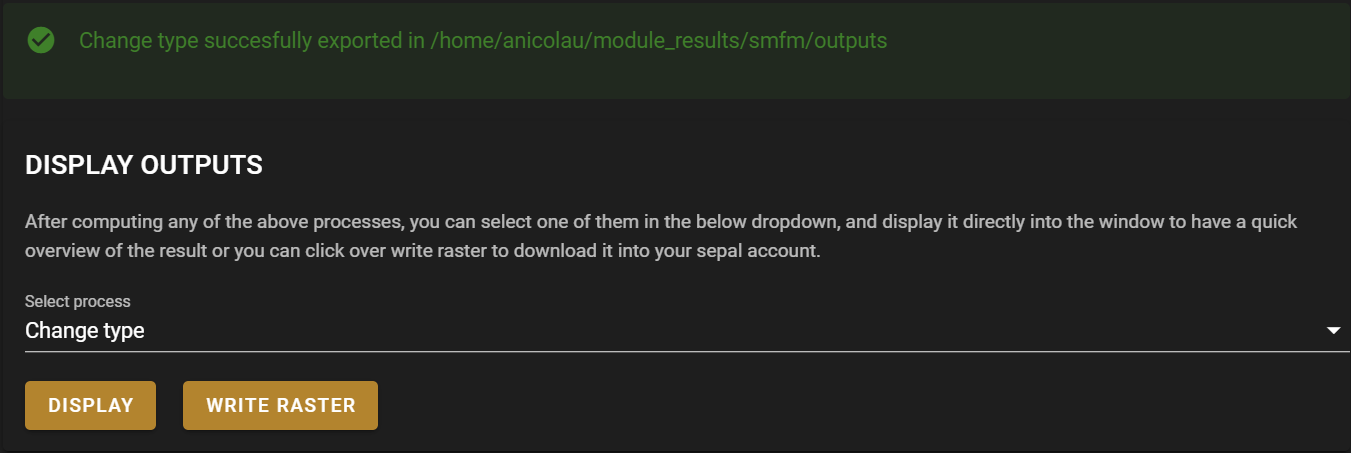
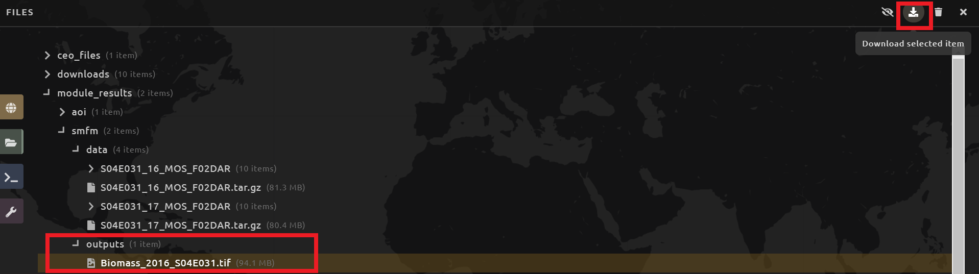
You can also use the Write raster option to save this map into your SEPAL account. Once you select Write raster, you should see a message in green informing you that your export has been completed.

The file will then be located in your SEPAL Files. You can download this map by selecting it and clicking the Download button in the upper-right corner. This will download the output as a TIF file that can be used in GIS software.

Here is a demonstration of the above steps:

Additional resources

On the left side, you can access:

• Source code: The source code of the tool, which is a GitHub repository.

• Wiki: The “README” file of the tool, where you can find additional information and instructions about how to use the tool.

• Bug report: The issue creation page on the GitHub repository of the tool, where you can report a bug or issue with using the tool.