

BFAST GPU#
GPU implementation of the BFAST algorithm to analyse time series
This article provides usage instructions for the GPU implementation of Breaks for Additive Seasonal and Trend (BFAST), implemented here as a Jupyter dashboard on SEPAL.
Introduction#
Large amounts of satellite data are now becoming available, which, in combination with appropriate change detection methods, offer the opportunity to derive accurate information on timing and location of disturbances (e.g. deforestation events across the Earth’s surface).
Typical scenarios require the analysis of billions of image patches/pixels, which can become very expensive from a computational point of view.
The BFAST package provides efficient, massively parallel implementation for one of the state-of-the-art change detection methods called BFASTmonitor <http://bfast.r-forge.r-project.org>, as proposed by Verbesselt et al.
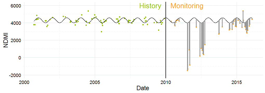
The analysis perfomed pixel-wise#
The implementation is based on OpenCL. It allows the processing of large-scale change detection scenarios given satellite time series data. The optimizations made are tailored to the specific requirements of modern, massively parallel devices, such as graphics processing units (GPUs).
The full documentation of the bfast package can be found on this page.
Usage#
Important
Before launching the BFAST module, you need to have at least one time series in your SEPAL folders.
Attention
If, while using the app, a user comes across an error starting with “Unable to allocate …”, it means that the instance used to run the application is too small. You’ll need to start a larger instance and restart the application.
Set up#
To launch the app, follow the steps to register for SEPAL.
Open a GPU instance in your terminal (g4 or g8).
Then move to the SEPAL Apps dashboard (purple wrench icon on the left side pane).
Finally, search for and select bfast GPU.
The application should launch itself in the BFAST process section. On the left side, the navdrawer will help you navigate between the different pages of the app. If you select wiki, bug report or code source, you will be redirected to the corresponding webpage.
Note
The launching process can take several minutes.
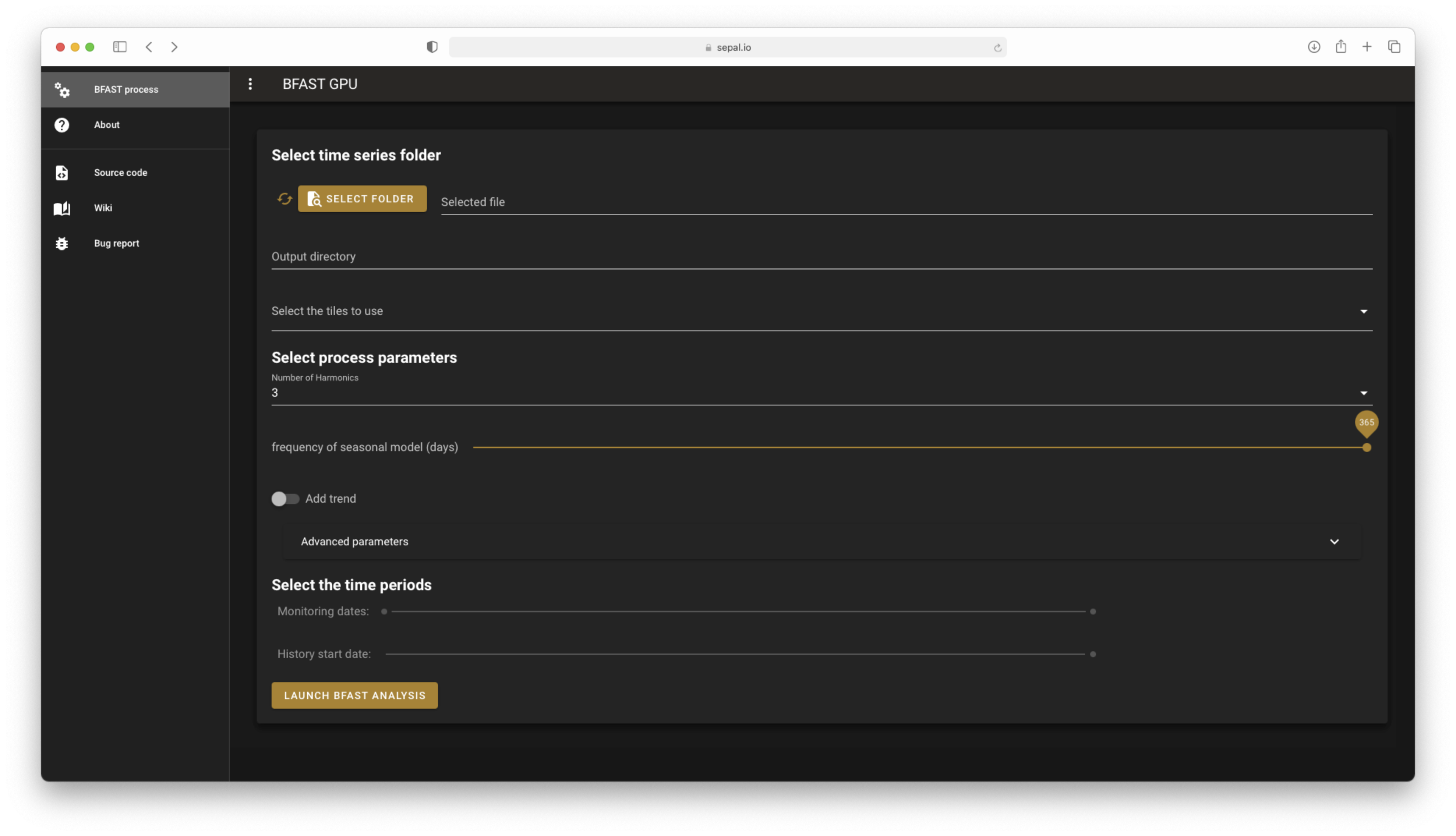
The landing page of bfast GPU#
Select folder#
Select a folder in the first widget.
Navigate through your folders to find the time series folder you want to analyse. Click outside the pop-up window to exit the selection. Your folder should only contain folders with numbered names (corresponding to each tile of the TS).
By selecting an appropriate folder, a widget will be automatically completed and enabled, as described below:
output directory name: Completed with the basename of your TS folder.select tiles to use: Preselect all available tiles.monitoring dates: The slider is enabled and completed with the date list included in the TS folder (the values default to the full range of dates).historical period: The slider is enabled and completed with the date list included in the TS folder (the value defaults to the first date of the TS).
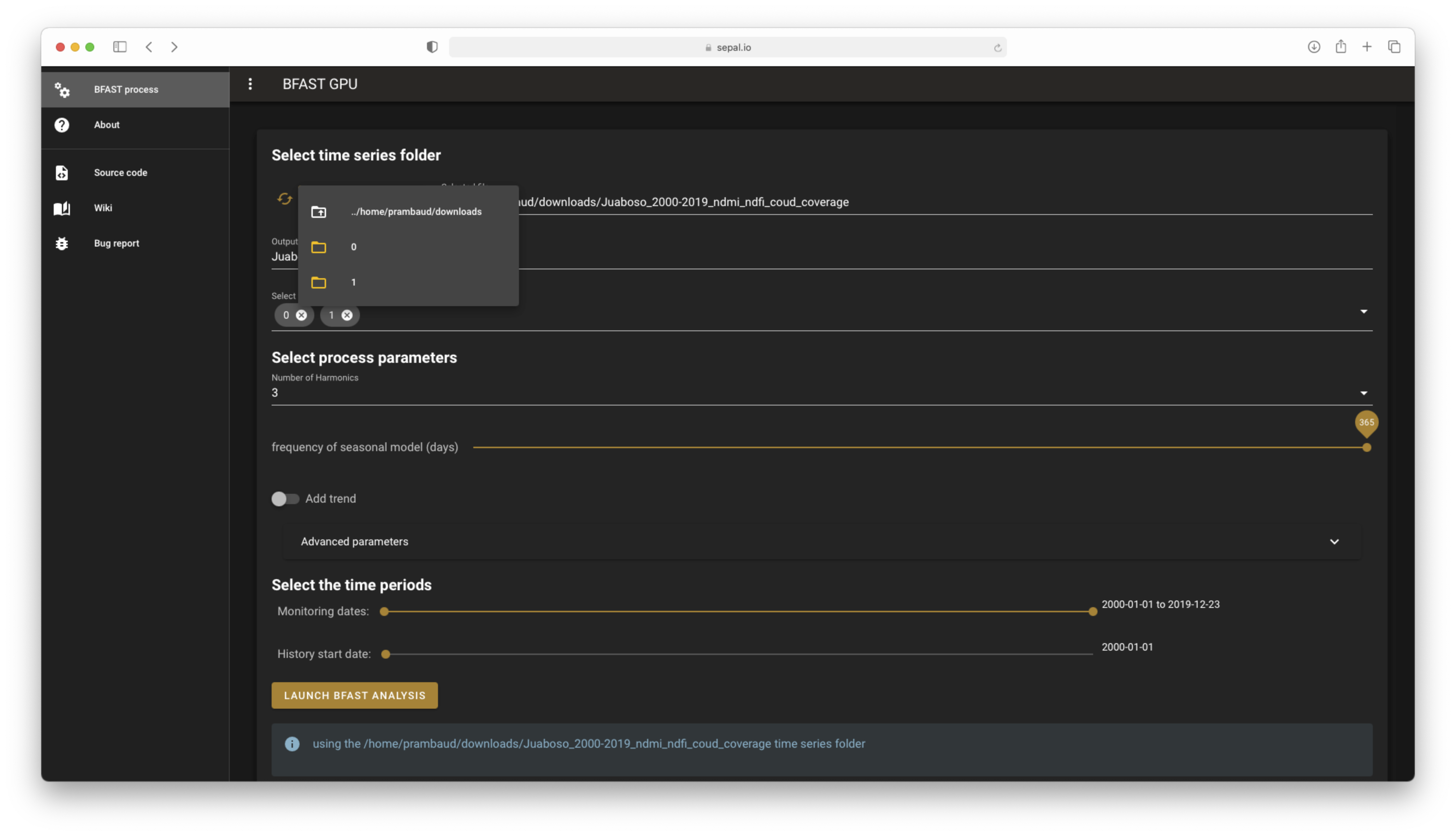
Select a folder and preload all information.#
Attention
If your selected folder does not meet the requirements of a SEPAL TS folder, the prefilled inputs will be emptied and disabled, and you will be notified twice that the folder is not set (in the input and in the warning banner). Select an appropriate folder to see these messages disappear.
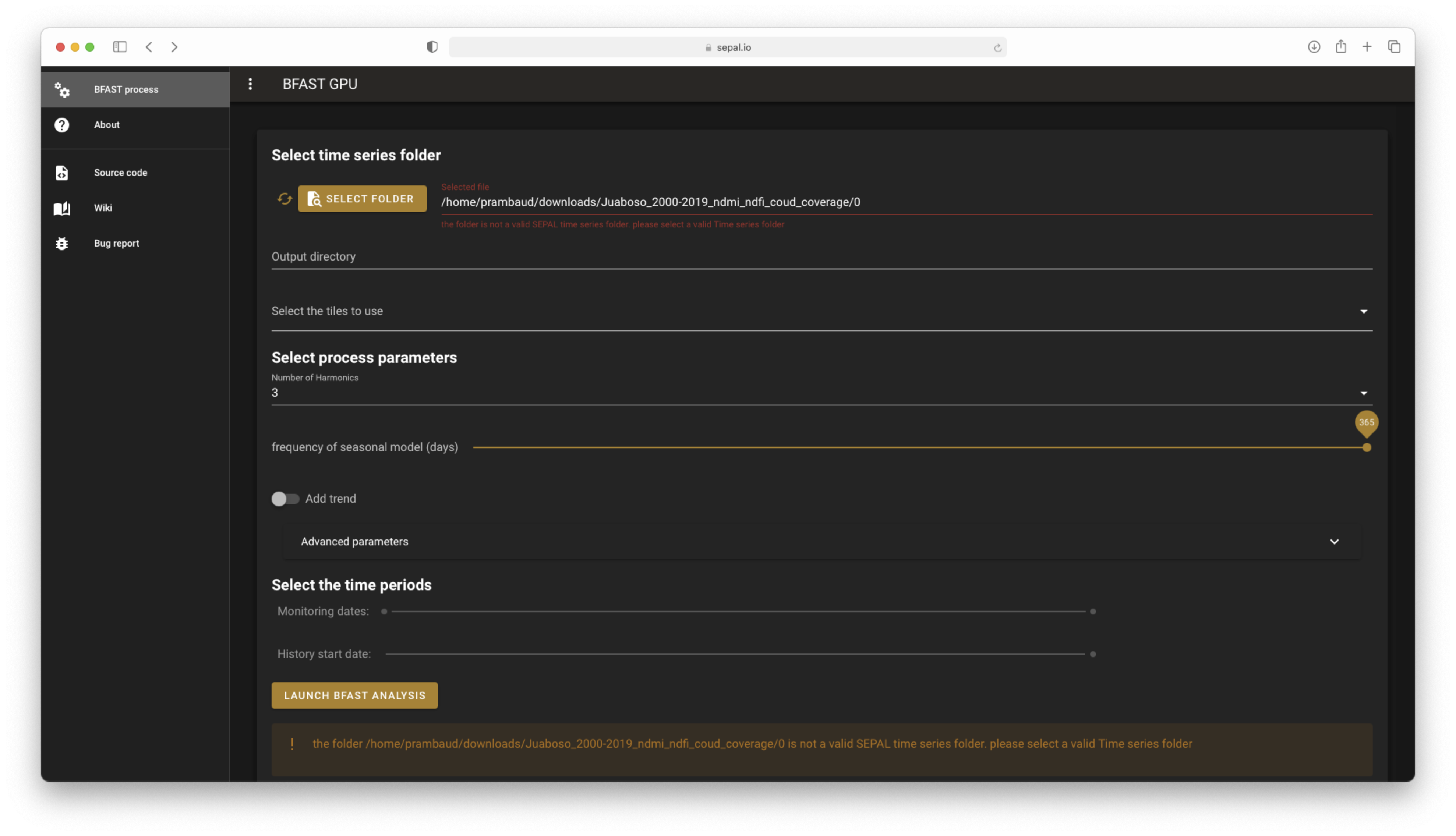
The error messages if incorrect folders are provided#
Parameters#
Now you can change the parameters to fit the requirements of your analysis:
output directory name: This name will be used to store all of your analysis. While it is completed automatically with the base name of your TS folder, you can change it.Note
The name of your folder can only contain alphanumeric characters and no special characters (e.g.
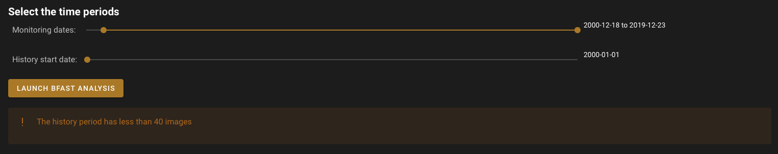
space). If you try to use them, the name will be automatically sanitized.Select tiles to use: These are the tiles that you want to use in your analysis. They default toallbut you can deselect any that you don’t need.Number of harmonic: Specifies the order of the harmonic term, defaulting to 3.Frequency of seasonal model: The frequency for the seasonal model, set here in months.Add trend: Whether a trend offset term shall be used or not.Monitoring dates: The year that marks the end of the historical period and the start of the monitoring period. The default value does not allow sufficient images in the historical stable period.Attention
If you allow less than 40 images between the start of the historical stable period and the start of monitoring, the programme will display a warning. You will still be able to launch the process, but the result will be very uncertain, as not enough images were provided to build an accurate model.
History start date: Specifies the start of the stable historical period
Advanced parameters#
Tip
These parameters are for advanced users only. The default value provides accurate results in many situations.
Select Advanced parameters and a new pane of options will be available:
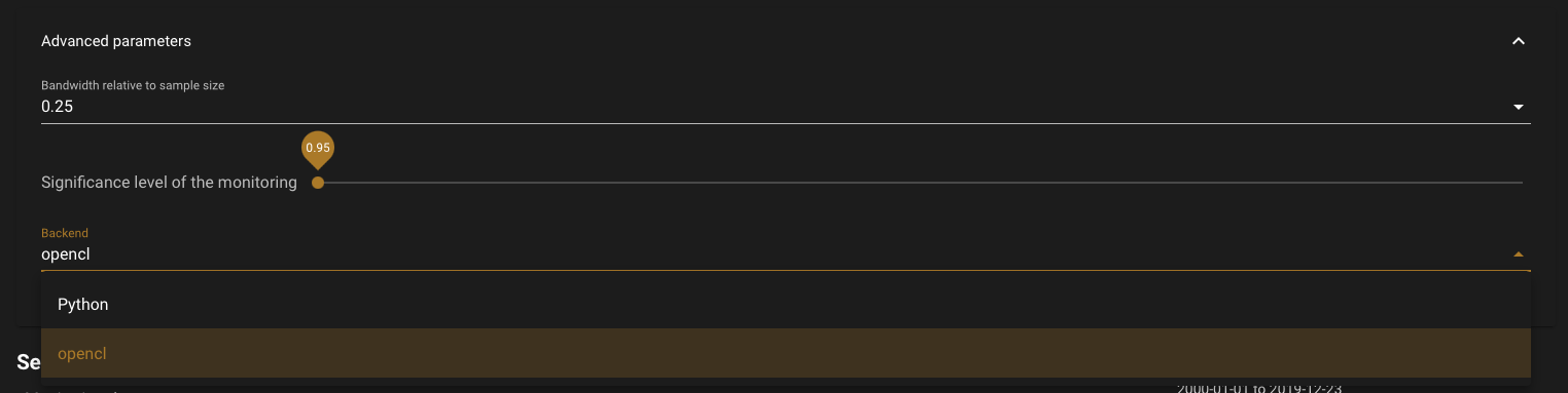
bandwith relative to sample size: Float in the interval (0,1), specifying the bandwidth relative to the sample size in the MOSUM/ME monitoring processes.Significance level of the monitoring: Significance level of the monitoring procedure and ROC, if selected (i.e. probability of Type I error).backend: Specifies the implementation that shall be used: Python resorts to the non-optimized Python version; OpenCL resorts to the optimized, massively parallel OpenCL implementation.Note
If you didn’t initiate a GPU instance before starting the application, the OpenCL backend will be disabled, as no GPU is available on your machine. Please close the app and your previous instance, and start a
g4org8. If you run the application on a GPU machine, the default backend is OpenCL.
Advanced parameters list#
Run process#
You can now select LAUNCH BFAST ANALYSIS to start the process.
The process will start shortly, notifying you of it’s advancement tile by tile in the Info banner, as shown in the following figure.
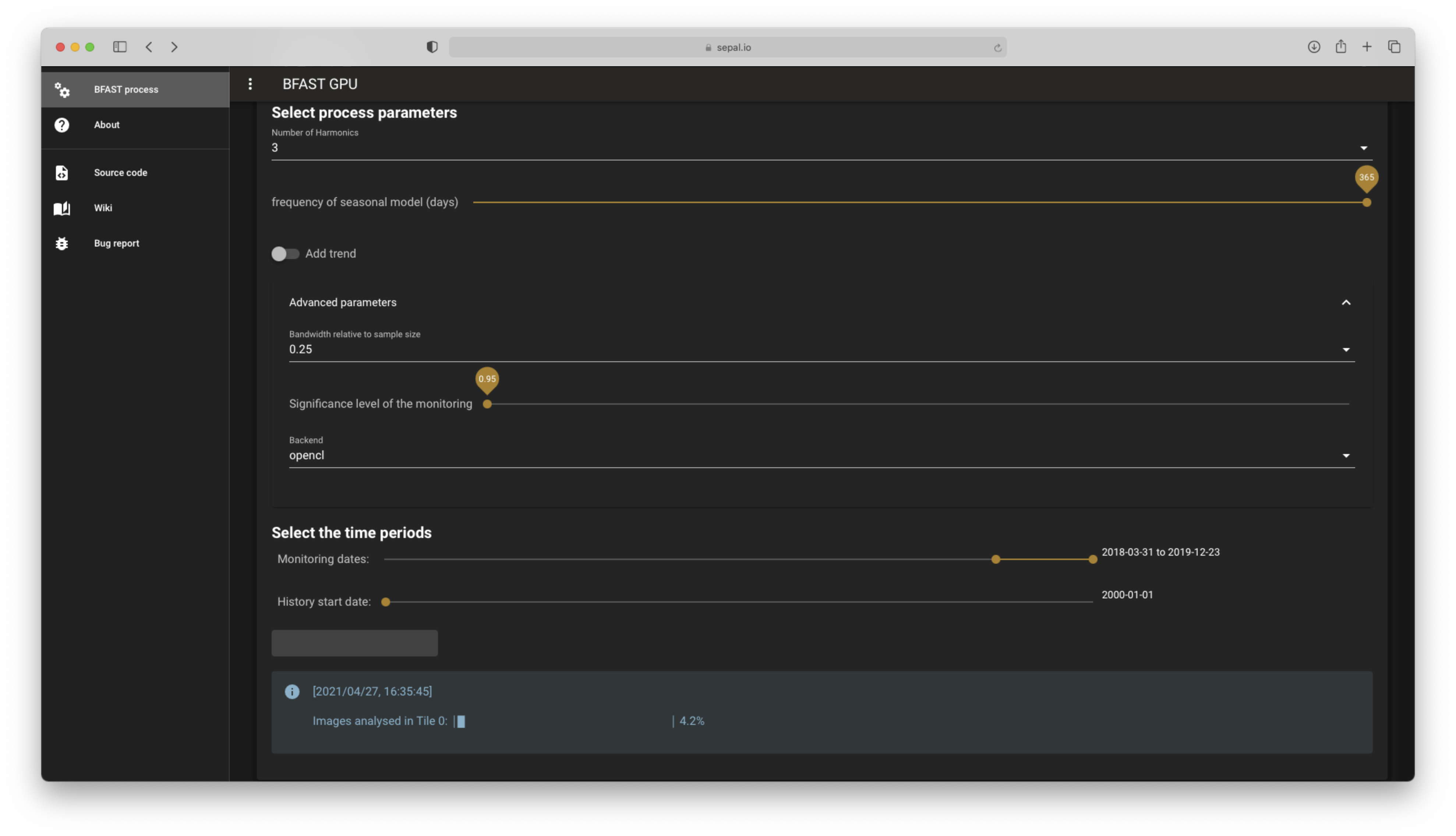
Process currently runnning#
Attention
Closing the app will shut down the Python kernel that runs underneath, thus stopping your process. In it’s current implementation, the app should stay open to run.
Tip
If your connection to SEPAL is lost and the application stops, use the exact same parameters as your previous analysis. The application will find the already computed tiles and images, and start from where it stopped instead of restarting from scratch.
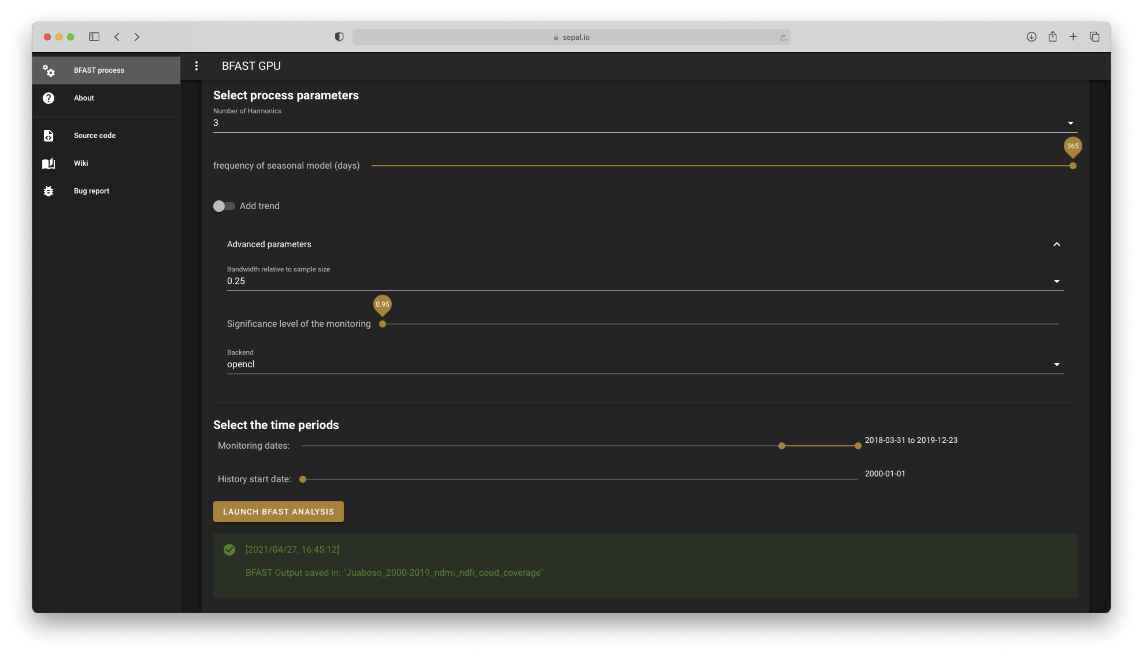
End of computation screen#
The module provided the following .vrt outputs:
- ~/module_results/bfast/[name_of_input]/[bfast_params]/bfast_outputs.vrt
It is a three-band raster:
Band 1: the breakpoints in decimal year format
Band 2: the magnitude of change
Band 3: the validity of the pixel model
This raster has the exact same dimensions as the input raster.
Example#
Here you’ll find an example of two bands over the Juaboso Region in Ghana with a monitoring period between 2017 and 2019:
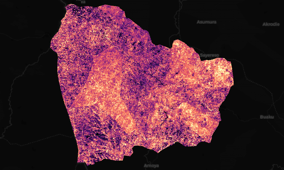
Magnitude display with the magma colormap, values in [-624, 417]#
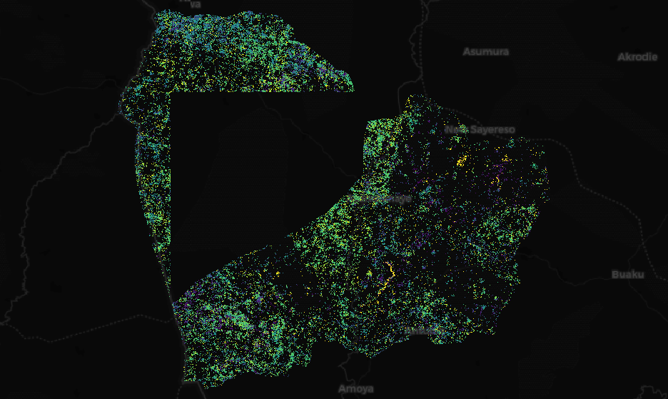
Breaks masked in the centre of the region, displayed with a viridis colormap, values in [2017.26, 2019.98]#