BFAST Explorer

Note

This tutorial comprehends the BFAST Explorer v0.0.1. Notice that if you are using a newer version, some features might be different.

Description

BFAST Explorer is a Shiny app, developed using R and Python, designed for the analysis of Landsat Surface Reflectance time series pixel data.

Three change detection algorithms - bfastmonitor, bfast01 and bfast - are used in order to investigate temporal changes in trend and seasonal components, via breakpoint detection.

If you encounter any bugs, please send a message to almeida.xan@gmail.com, or create an issue on the GitHub page.

Tutorial

Albeit very simple, please follow this short usage guide to learn how to properly use the tool.

Map Tab

This is the starting tab, which we first see when we run the tool. The tab is composed of an interactive map (rendered using Google Maps engine) and a navigation toolbar. Feel free to zoom and pan the map.

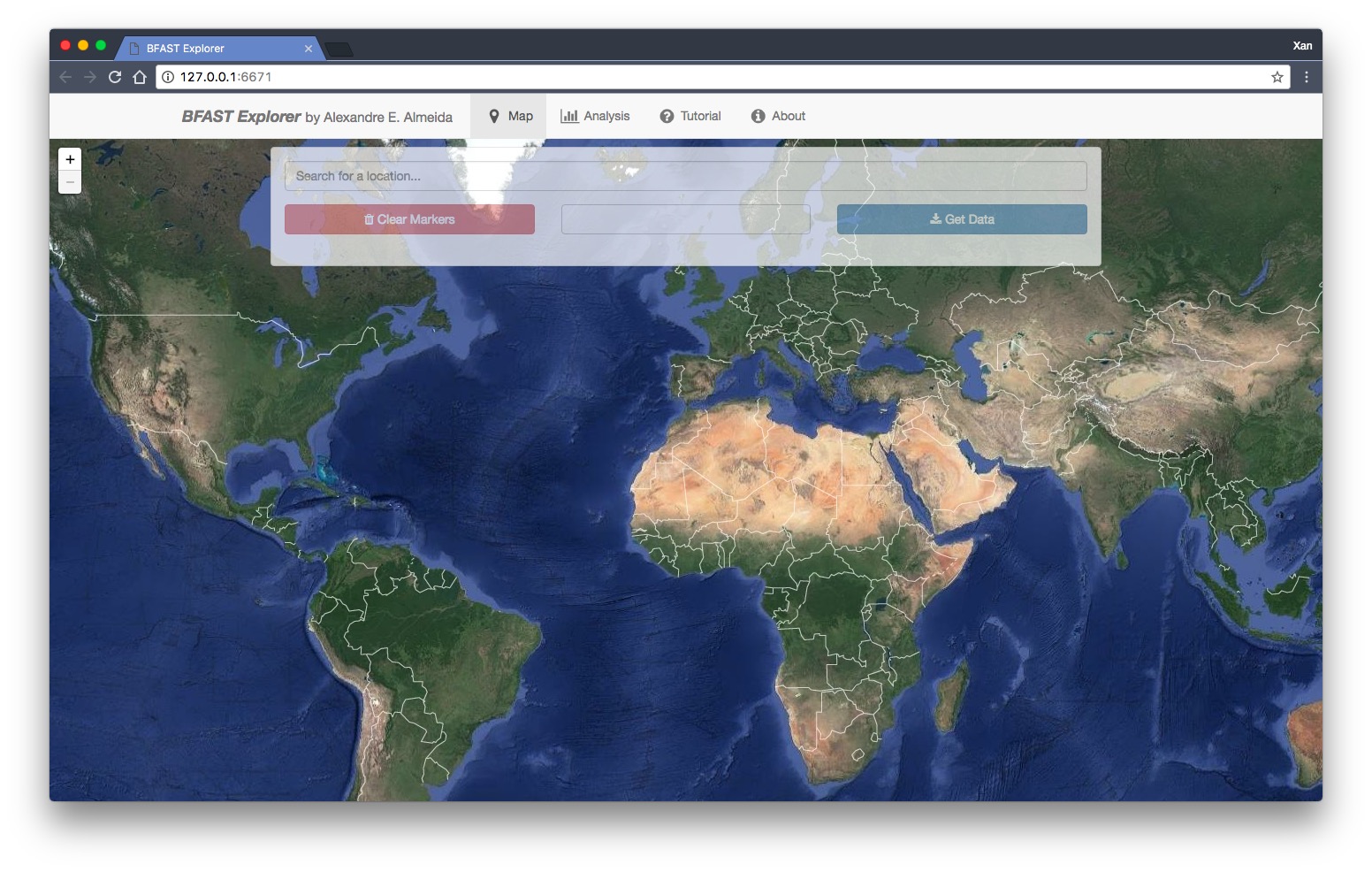
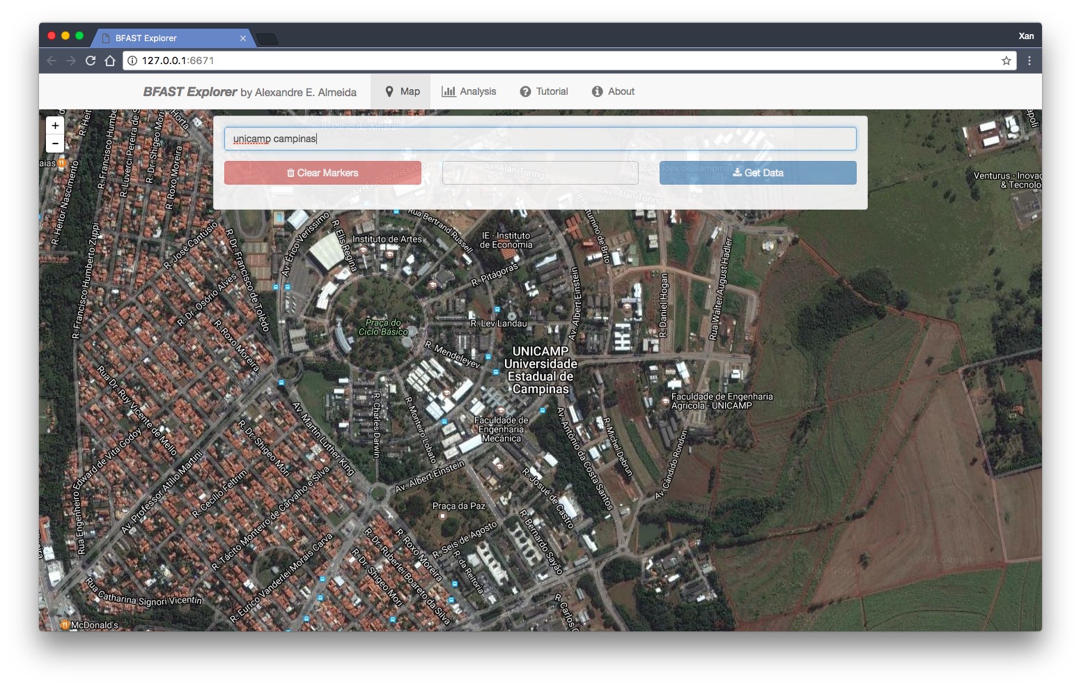
If we wish, we can also use the search field located on the top of the toolbar to search for a location. Then, the map automatically zooms to the desired location, similar to how Google Maps works. In the example, we searched for unicamp campinas, which is the University of Campinas.

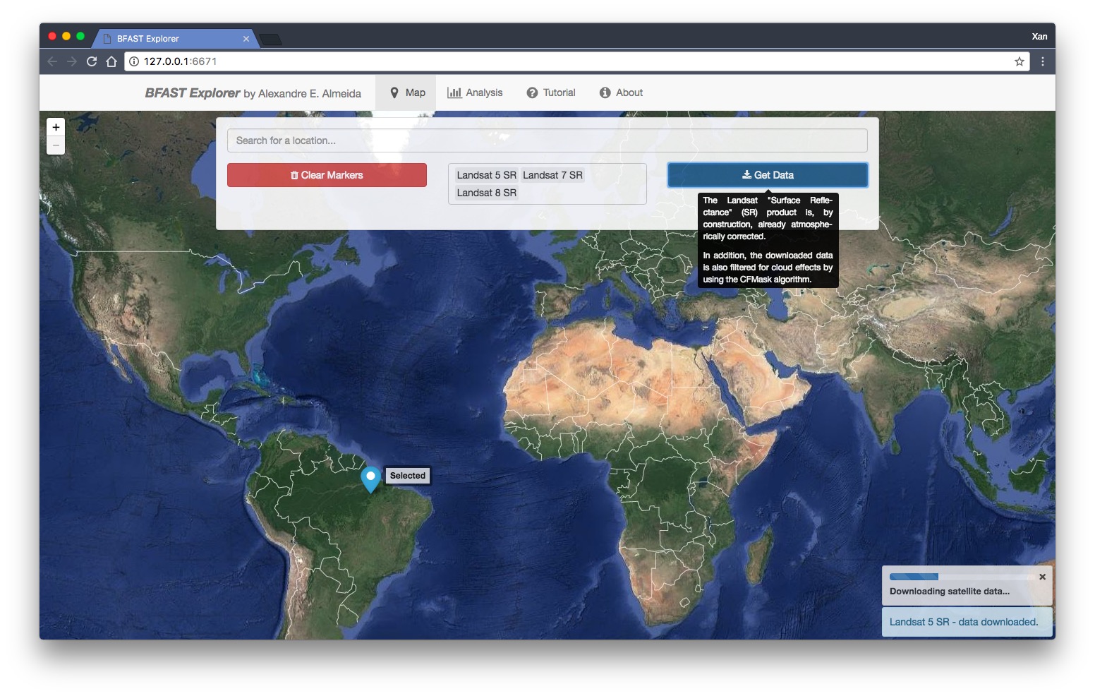
Now, let’s zoom out all the way back and place a marker at the north of Brazil, as shown. To place a marker, simply click on the map. If we want to, we can also place multiple markers.

We may also wish to clear all the placed markers. To do that, click on the red button on the left side of the toolbar.

After that, we need to select one of the markers in order download its Landsat pixel data. To do that, simply click on an already placer marker, and it will be highlighted. Only one marker may be selected at a time.

By selecting a marker, we can now choose a combination of which satellites to download from using the drop-down menu, located on the bottom of the toolbar. For instance, let’s choose all the available satellites products: Landsat 5, 7 and 8 SR.

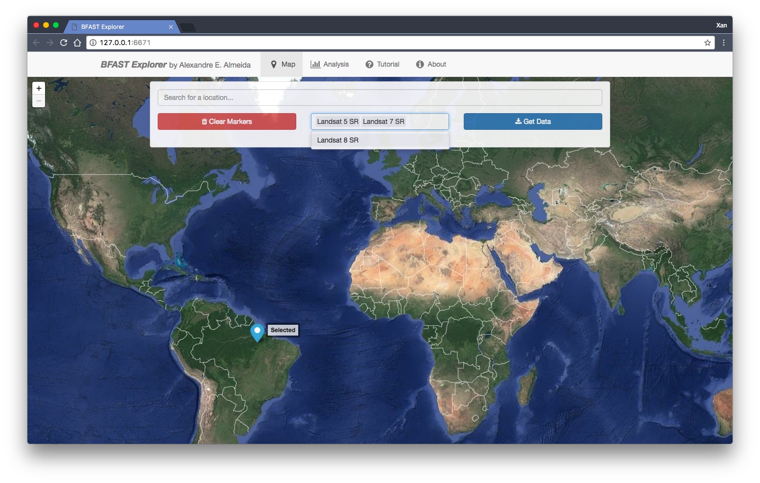
Then, we press the Get Data blue button, located on the right side of the toolbar. By pressing that button, the download will start. We can keep track of the download progress by looking to the lower right corner. All the historical data available are downloaded, which should take less than 10 seconds for the three productsselected.

Note

As of the writing of this guide, not all Surface Reflectance data are availble from GEE. So, depending on where we place our markers, we may face a message indicating that ‘No data available for the chosen satellite(s) and/or region… Please change your query and try again.’. Since we rely heavily on GEE to download the data, there’s nothing we can do yet. We’re sorry for that.

If the download is successful, we’ll receive a message directing to the Analysis tab.

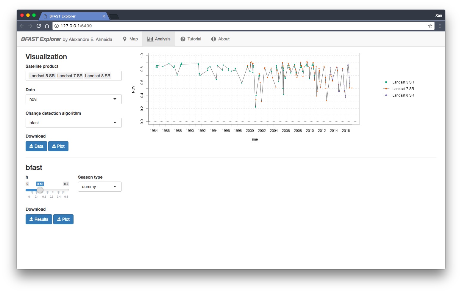
Analysis Tab

In this tab, we can analyze the downloaded data and, then, locally save the results as files.

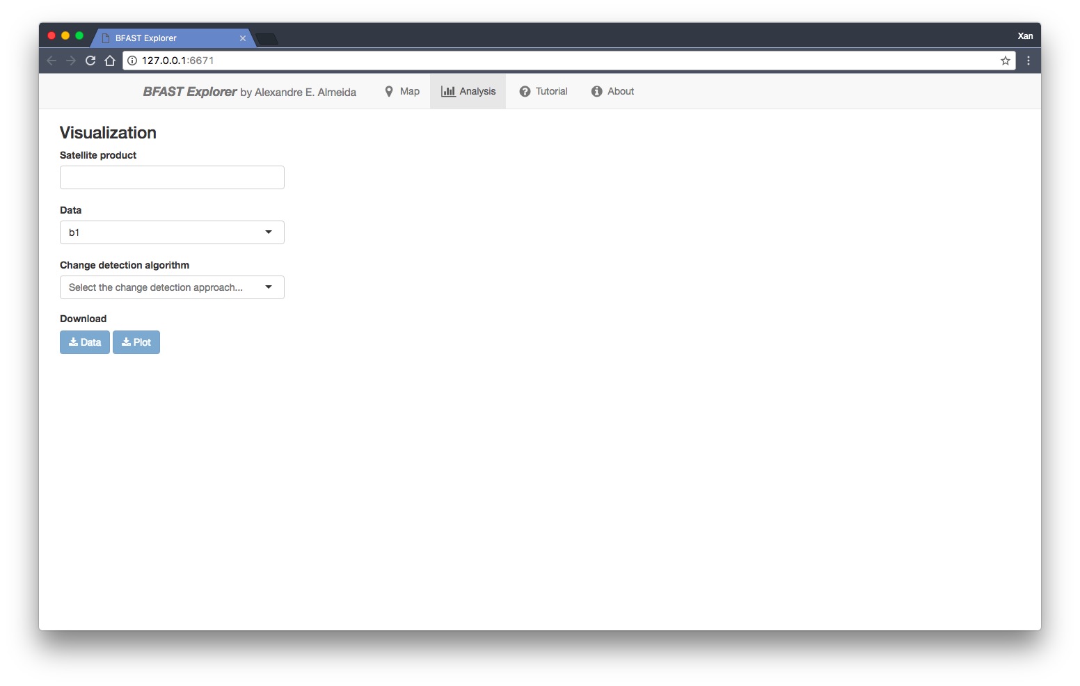
First, let’s choose which satellite time series date to visualize. Note that, even though we downloaded data from Landsat 5, 7 and 8 SR, we’re can still analyze them separately. However, let’s proceed by choosing all of them.

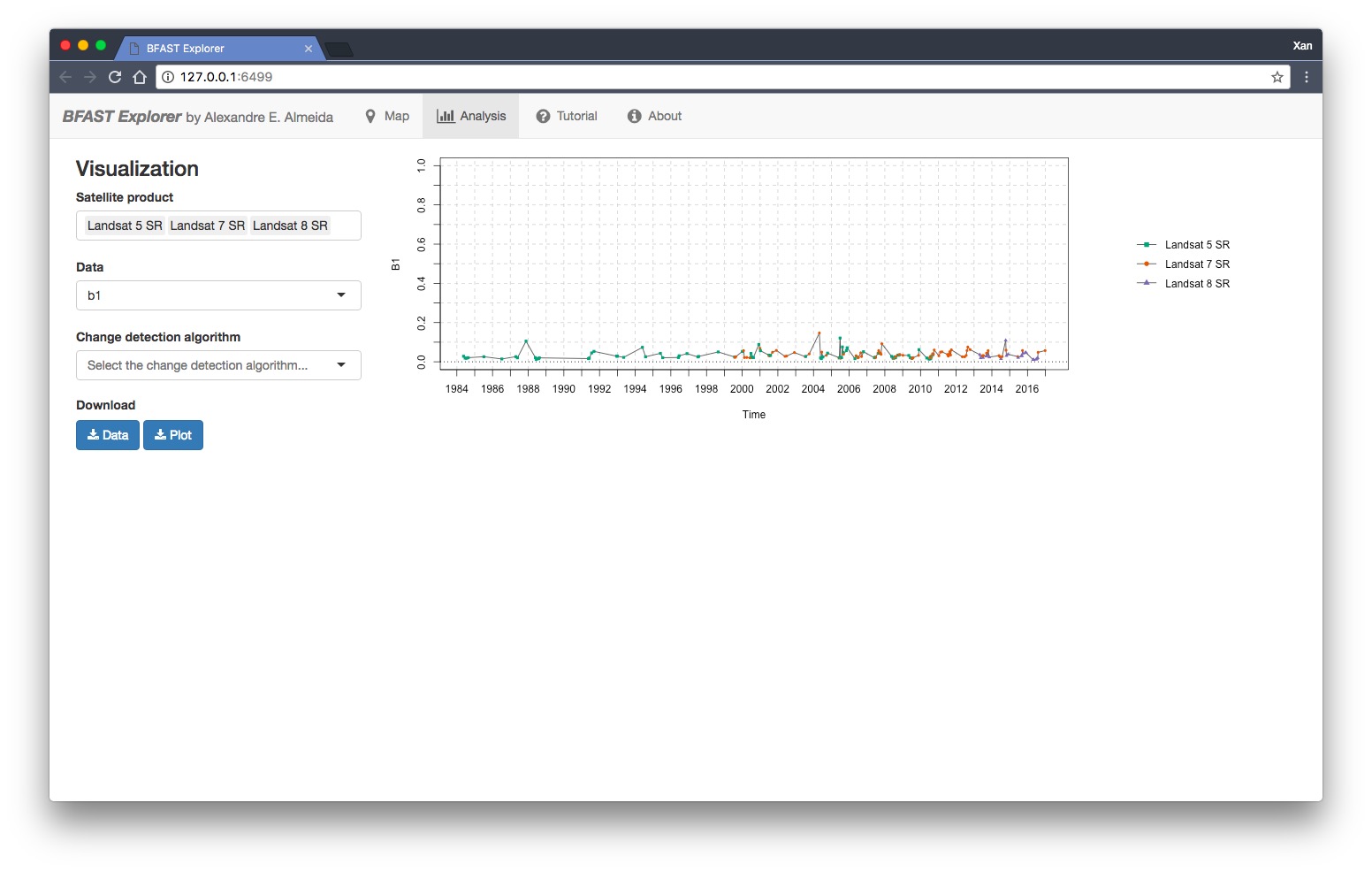
As we can see, the time series of the first spectral band (b1) is plotted for all satellites. A colored legend distinguishes the different sources.

Note

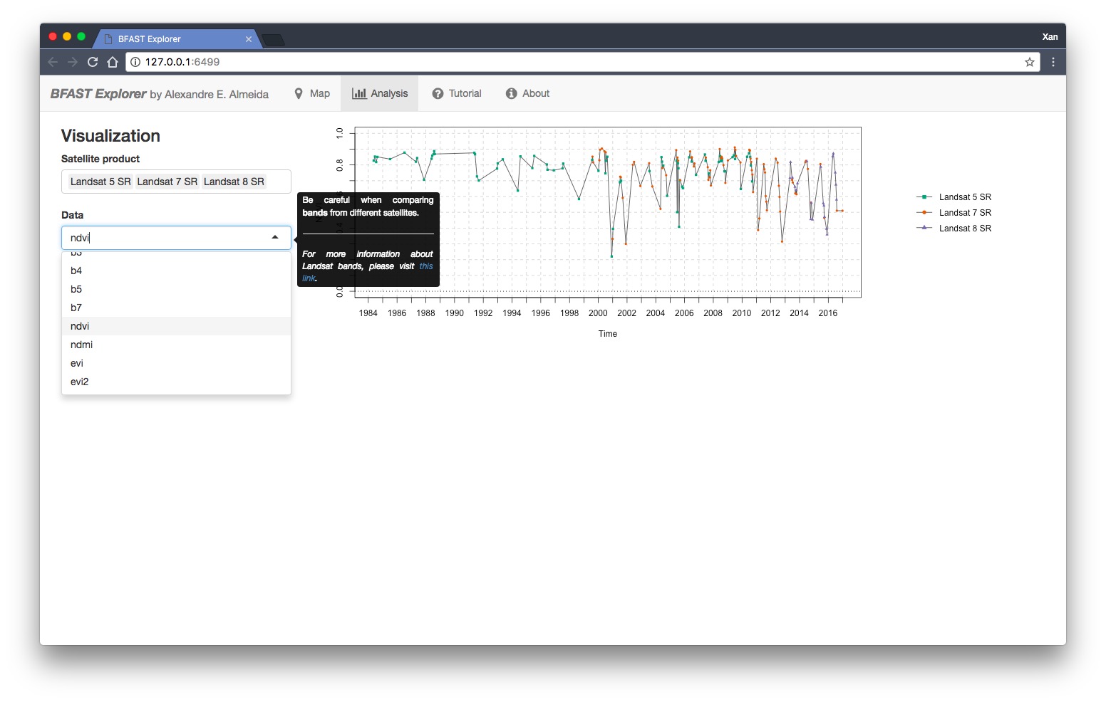
be careful when comparing spectral bands data from different satellites, as they may not correspond to the same wavelength range! Read more about this here.

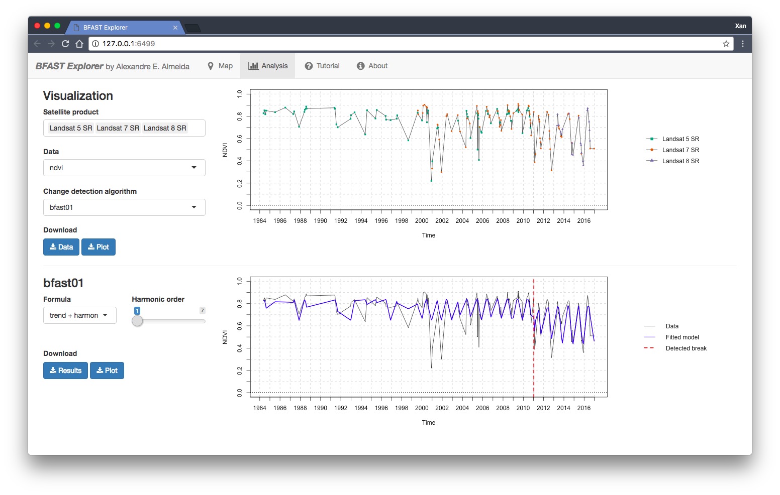
Apart from the spectral bands, there are also four spectral-bands-derived indexes available: NDVI, NDMI, EVI and EVI2. Let’s check, for example, the NDVI time series.

If we want to, we can also download all the time series data as a file. To do that, press the Data blue button. All the data will be downloaded as a .CSV, ordered by the acquisiton date. Also, an additional column is included, in order to distinguish the satellite sources.

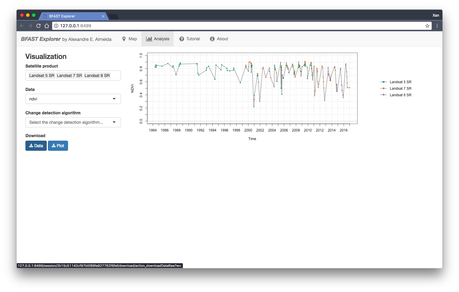
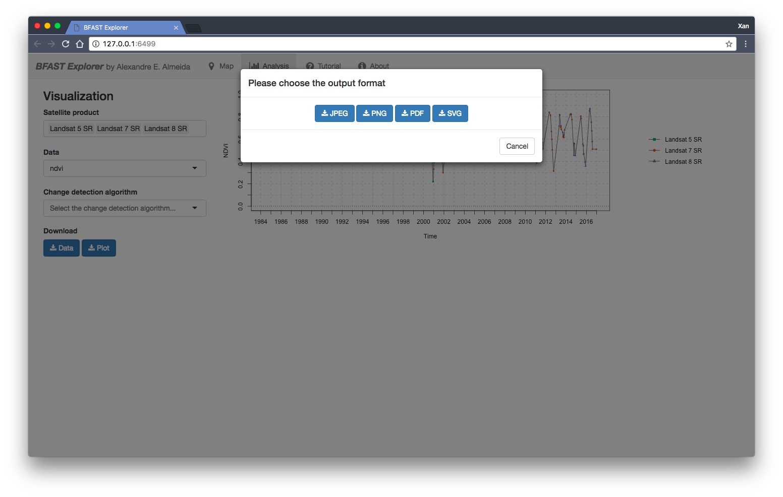
We may download the time series plot as an image, by pressing the Plot blue button. A window will appear offering some raster (.JPEG, .PNG) and a vectorial (.SVG) image output formats.

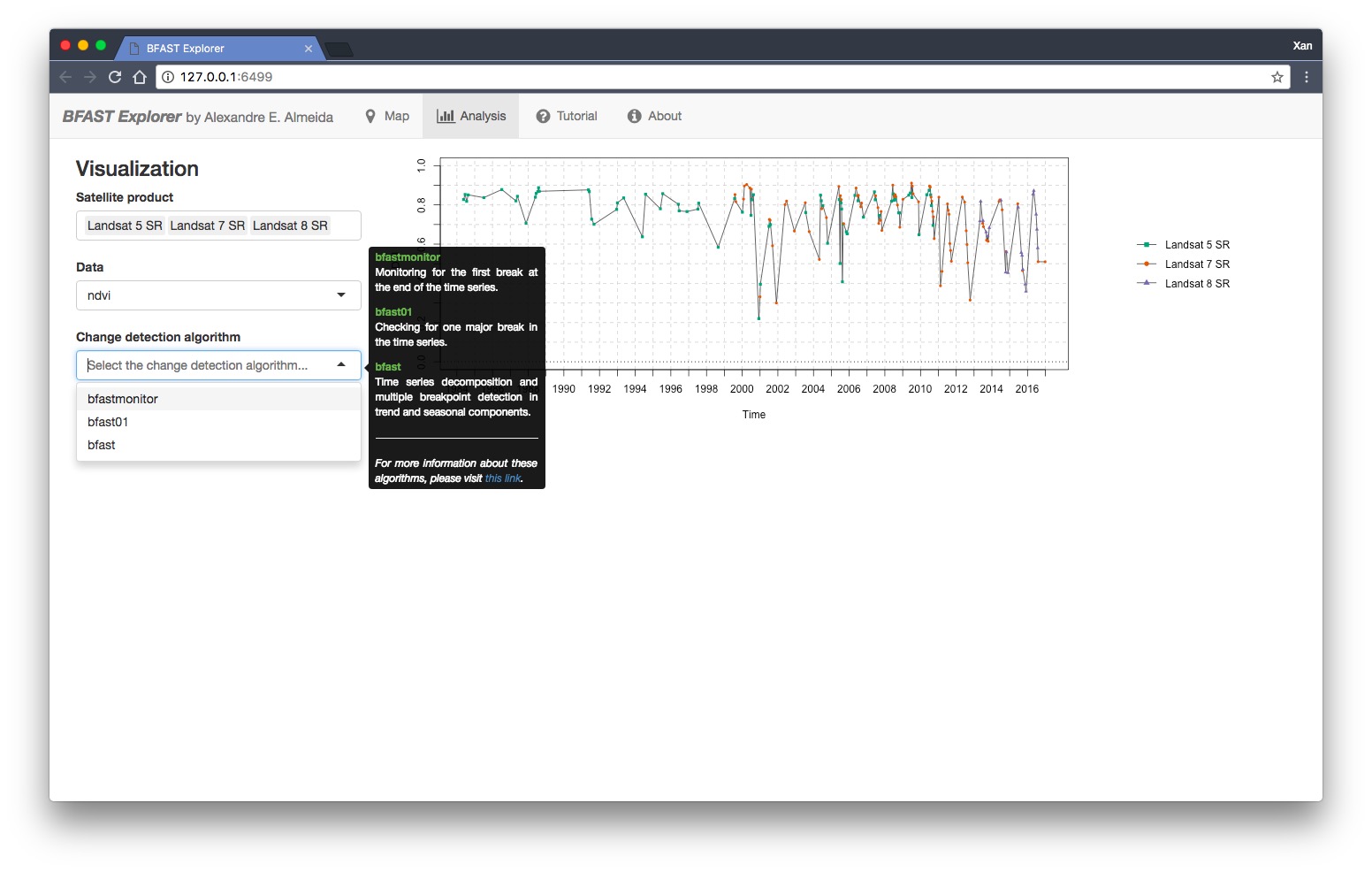
Next, we select the change detection algorithm. Three options are available: bfastmonitor, bfast01 and bfast. More information about these algorithms can be found here.

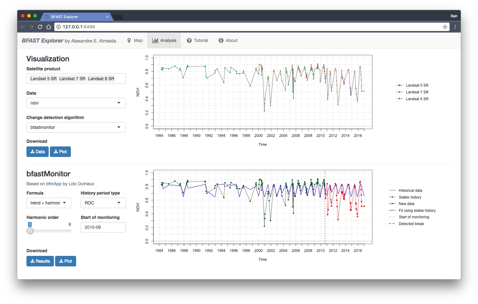
By selecting bfastmonitor, we are able to tweak four parameters on the left side-bar: formula, history period type, harmonic order, and start of monitoring. These parameters have different impacts on the results, which can be verified on the right side plot. Here, we set the maximum value of the harmonic order to 9 to avoid some problems.

Similar to the time series, we can also download the results of the change detection algorithms as .RDS data files, by clicking on the Results blue button. If we wish to download the plot, we can press the Plot blue button.

For more information on how to load .RDS files on R, please check this link.

By selecting bfast01, we can tweak two parameters: formula, and harmonic order.

Here, the maximum value of the harmonic order is dynamically set depending on the time series data length and the choice of the formula parameter.

Finally, by selecting bfast, we may tweak two parameters: h (minimal segment size), and season type. Please note that, since bfast can detect multiple breakpoints, it may take a couple of seconds to process, in comparison to the previous two algorithms.