

se.plan#
Generate information on forest restoration potential to support forest restoration planning decisions with se.plan
Introduction#
Overview#
se.plan is a spatially explicit online tool designed to support forest restoration planning decisions by restoration stakeholders.
Part of System for Earth Observation Data Access, Processing and Analysis for Land Monitoring (SEPAL), a component of the free, open-source software suite, Open Foris from the Food and Agriculture Organization of the United Nations (FAO), se.plan aims to identify locations where the benefits of forest restoration are high relative to restoration costs, subject to biophysical and socioeconomic constraints that users impose to define the areas where restoration is allowable. The computation is performed using cloud-based supercomputing and geospatial datasets from Google Earth Engine (GEE) available through SEPAL.
As a decision-support tool, se.plan is intended to be used in combination with other information users may have that provides greater detail on planning areas and features of those areas that the tool might not adequately include. It offers users the option to replace its built-in data layers, which are based on publicly available global datasets, with users’ own customized layers (see Primary data sources for a list of the tool’s built-in data layers and their sources).
The following sections highlight key features of se.plan.
Following the three steps below, the tool can be used to generate information on forest restoration potential.
To generate maps and related information on restoration’s benefits, costs and risks for all suitable sites within the planning area:
Select your geographical planning area.
Rate the relative importance of different restoration benefits from your perspective.
Impose constraints that limit restoration to only those sites viewed as suitable (related to ecological and socioeconomic risks).
In addition to reading this article, the SEPAL team encourages users to watch the following video:
Geographical resolution and scope#
se.plan divides the Earth’s surface into grid cells with 30 arc-second resolution (approximately 1 km at the equator).
The tool only includes grid cells that satisfy the following four criteria (view in GEE):
They are in countries or territories of Africa and the Near East, Asia and the Pacific, and Latin America and the Caribbean that the World Bank classifies as low- or middle-income countries or territories (LMICs) during most years of the 2000–2020 period. There are 139 countries and territories in total and can be found in the section, Countries.
They include areas where tree cover can potentially occur under current climatic conditions, as determined by Bastin et al. (2019).
Their current tree cover, as measured by the European Space Agency’s Copernicus Programme (Buchhorn et al. 2020), is less than their potential tree cover.
They are not in urban use.
se.plan labels grid cells that satisfy these criteria as potential restoration sites. It treats each grid cell as an independent restoration planning unit, with its own potential to provide restoration benefits and entail restoration costs and risks.
Methodology#
Selection of planning area#
se.plan offers users multiple ways to select a planning area, which the tool labels as Area of interest (AOI) as described in the Usage.
Restoration benefits#
In its current form, se.plan provides information on four benefits:
biodiversity conservation
carbon sequestration
local livelihoods
wood production
se.plan includes two indicators each for biodiversity conservation and local livelihoods, and one indicator each for carbon sequestration and wood production. Each indicator is associated with a data layer that estimates each grid cell’s relative potential to provide each benefit if the grid cell is restored; the relative potential is measured on a scale of 1 (low) to 5 (high) (see Data layers for benefits for more information on the interpretation and generation of data layers for the benefit indicators).
Users rate the relative importance of these benefits from their standpoint (or the standpoint of stakeholders they represent). Then, se.plan calculates an index that indicates each grid cell’s relative restoration value aggregated across all four benefit categories. This restoration value index is a weighted average of the benefits with user ratings serving as the weights. It therefore accounts for not only the potential of a grid cell to provide each benefit, but also the relative importance that a user assigns to each benefit. It is scaled from 1 (low restoration value) to 5 (high restoration value) (see Benefit–cost ratio for more information on the generation of the index).
Restoration cost#
Forest restoration incurs two broad categories of costs, opportunity cost and implementation costs.
Opportunity cost refers to the value of land if it is not restored to forest. se.plan assumes that the alternative land use would be some form of agriculture (either cropland or pasture). It sets the opportunity cost of potential restoration sites equal to the value of cropland for all sites where crops can be grown, with the opportunity cost for any remaining sites set equal to the value of pasture. Sites that cannot be used as either cropland or pasture are assigned an opportunity cost of zero.
Implementation costs refer to the expense of activities required to regenerate forests on cleared land, including both:
initial expenses incurred in the first year of restoration (Establishment costs), which are associated with such activities as site preparation, planting and fencing; and
expenses associated with monitoring, protection and other activities during the subsequent three to five years that are required to enable the regenerated stand to reach the “free to grow” stage (Operating costs).
se.plan assumes that implementation costs include planting expenses on all sites. This assumption might not be valid on sites where natural regeneration is feasible. To account for this possibility, the tool includes a data layer that predicts the variability of natural regeneration success.
se.plan calculates the overall restoration cost of each site by combining the corresponding estimates of the Opportunity cost and Implementation costs (see Cost data layers for more information on the interpretation and generation of the data layers for opportunity and implementation costs).
Benefit–cost ratio#
se.plan calculates an approximate benefit–cost ratio for each site by dividing the restoration value index by the restoration cost and converting the resulting number to a scale from 1 (small ratio) to 5 (large ratio). Sites with a higher ratio are the ones that the tool predicts are more suitable for restoration, subject to additional investigation that draws on other information users have on the sites (see Benefit–cost ratio for more information on the generation and interpretation of this ratio).
A key limitation is that the ratio does not account for interdependencies across sites related to either benefits, such as the impact of habitat scale on species extinction risk, or costs, such as scale economies in planting trees. This limitation stems from the tool’s treatment of each potential restoration site as an independent restoration planning unit.
Constraint#
se.plan allows users to impose constraints that limit restoration to only those sites they view as suitable, in view of ecological and socioeconomic risks. It groups the constraints into four categories:
Biophysical, including elevation, slope, annual rainfall, baseline water stress and terrestrial ecoregion;
Current land cover, including shrubland, herbaceous vegetation, agricultural land, urban/built up, bare/sparse vegetation, snow and ice, herbaceous wetland, and moss and lichen;
Forest change, including deforestation rate, climate risk and natural regeneration variability; and
Socioeconomic, including protected areas, population density, declining population, property rights protection, and accessibility to cities.
se.plan enables the user to adjust the values that will be masked from the analysis for most of these constraints. Some of the constraints are binary variables, with a value of 1 if a site has the characteristic associated with the variable and 0 if it does not. For these constraints, users can choose if they want to keep zeros or ones. (See Constraints data layers for more information on the interpretation and generation of the data layers for the constraints.)
Customization#
Constraints, costs and indicators are based on layers provided within the tools. These layers may not cover the AOI selected by the user, or may provide less accurate/up-to-date data than national datasets available. To allow users to improve the quality of the analysis, se.plan provides the possiblity of replacing these datasets by any layer available with GEE.
(See the Usage section for more information on the customization process.)
Output#
se.plan provides two outputs:
A map of the restoration suitability index scaled from 1 (low suitability) to 5 (high suitability). This map, generated within the GEE API can be displayed in the app but also exported as a GEE asset or a
.tiffile in your SEPAL folders.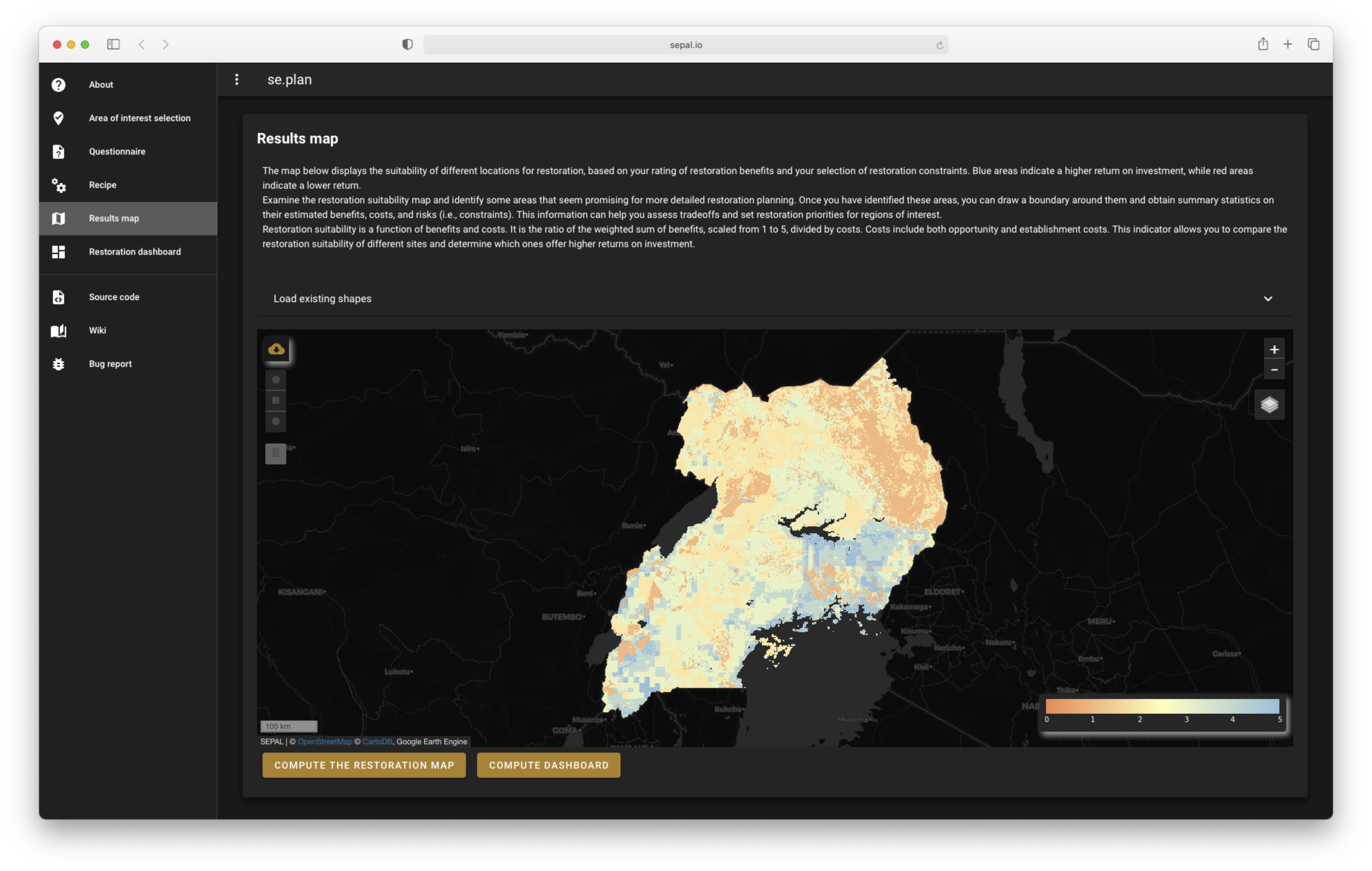
A dashboard gathering information on the AOI and sub-AOIs defined by the user. The suitability index is thus presented as surfaces in mega hectares (Mha), but se.plan also displays the mean values of the benefits and the sum of all the used constraints and cost over the AOIs.
Usage#
In this section, we will exaustively describe how to use the se.plan application.
Open the app#
To access the application, open your SEPAL account by going to https://sepal.io.
Then, select the purple wrench on the right side of your screen to access the Apps dashboard (https://sepal.io/app-launch-pad). All available SEPAL applications are displayed on this page.

In the Apps dashboard, enter se.plan in the search bar. The list of applications should be reduced to one.
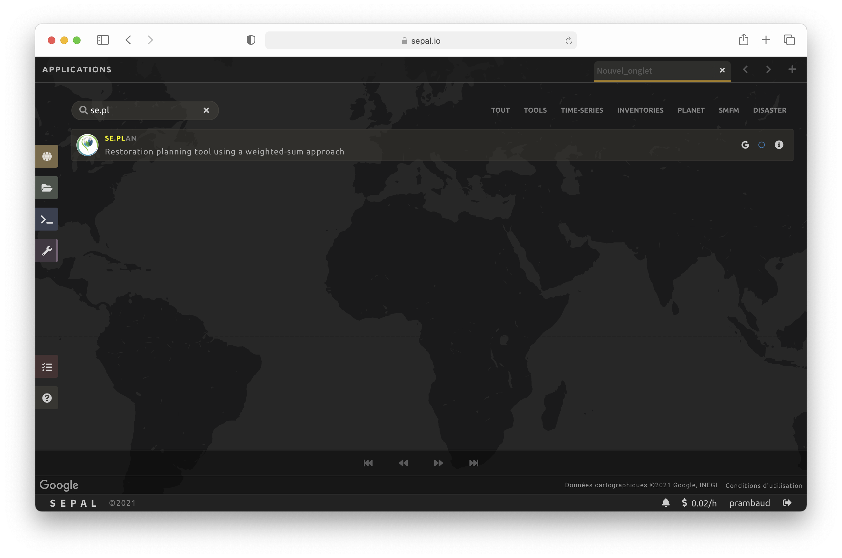
Select the se.plan app and wait until the loading is finished. The application will display the About page.
Note
You might need to manually start an instance that is more powerful than the default t1 instance (see the Module <../module/index.html>`__ section to learn how to start instances).

Use the drawers on the left to navigate through the application panes.
The next sections will guide you through each step of the se.plan process.
Select AOI#
The Restoration suitability index (referred to as Index) will be calculated based on user inputs.
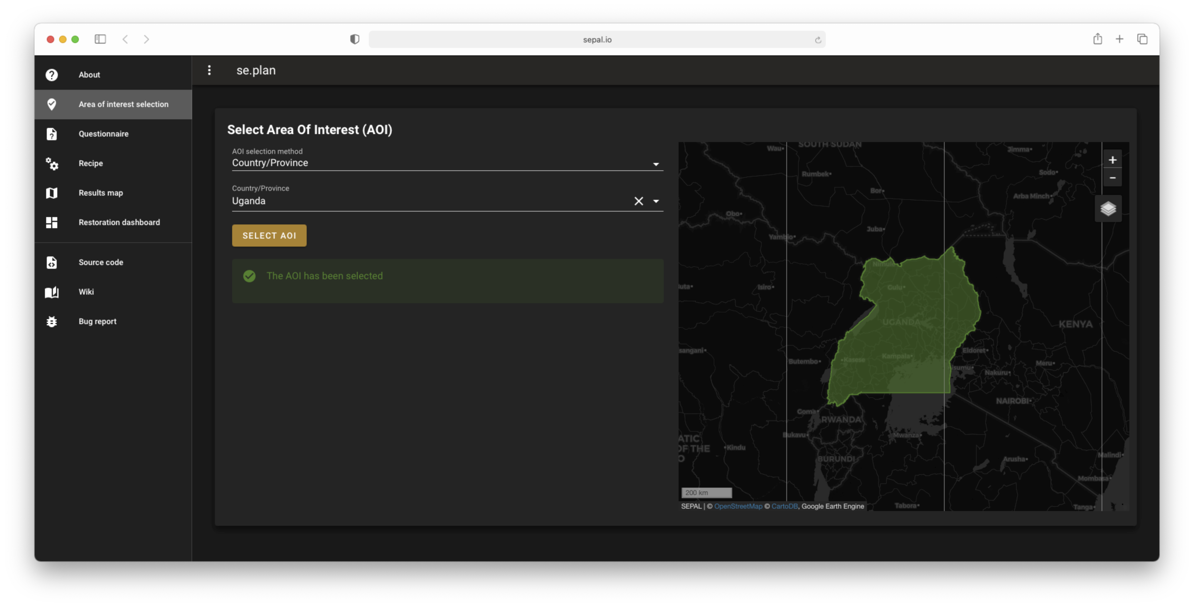
The first mandatory input is the AOI. In this step, you’ll have the possibility to choose from a predefined list of administrative layers or use your own datasets. Available options include:
Predefined layers
Country/province
Administrative level 1
Administrative level 2
Custom layers
Vector file
Drawn shapes on map
GEE asset
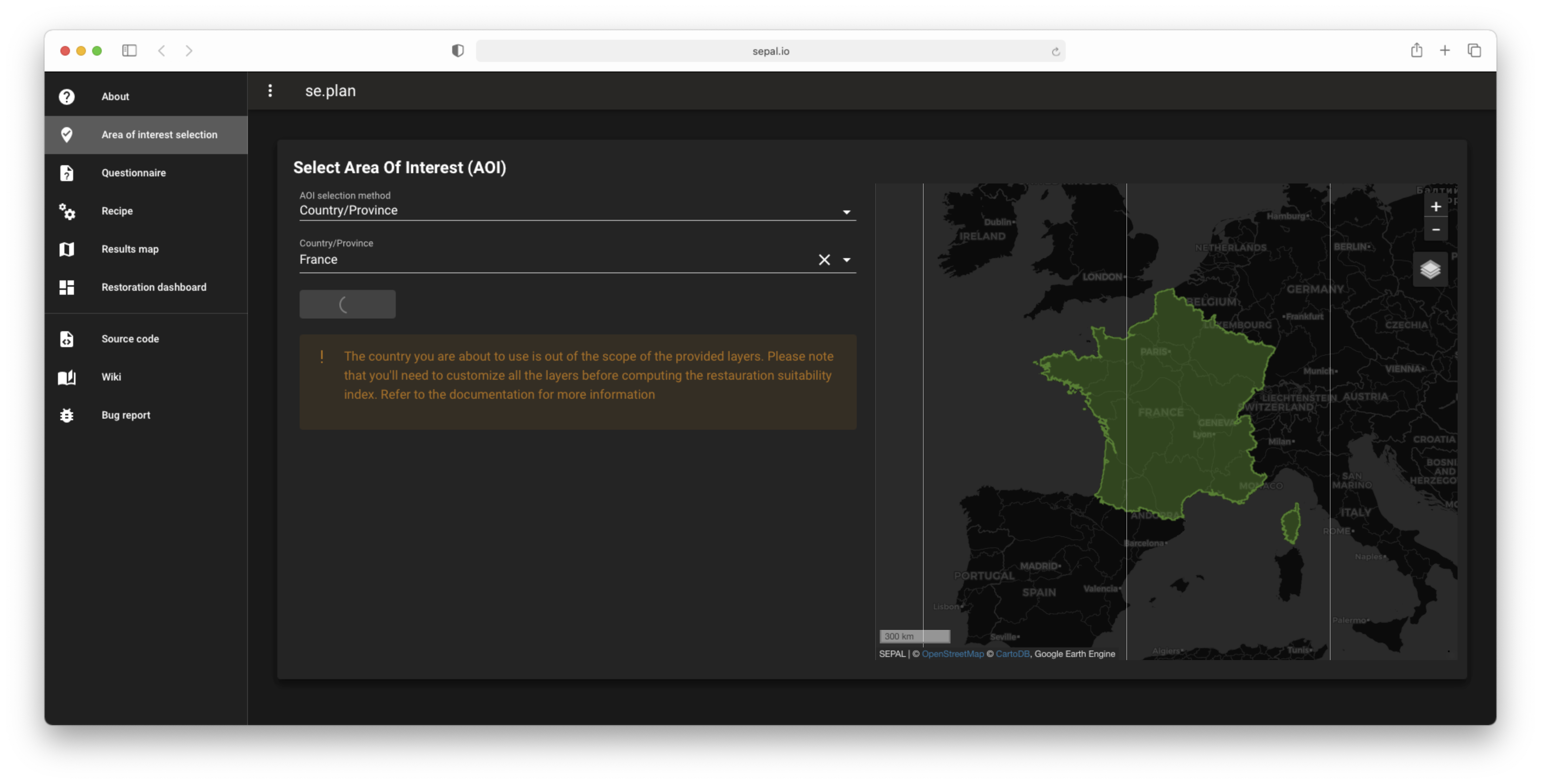
After selecting the desired area, select the Select these inputs button; the map will display your selection. Once you see the green confirmation message, select the Questionnaire pane to move to the next step.
Note
You can only select one AOI. In some cases, depending on the input data, you could run out of resources in GEE.
Attention
As described in the first section of this article, the layers provided in this application cover the 139 countries defined as LMICs by the World Bank. If the selected AOI is out of these boundaries, the provided layers cannot be used to compute the Index. A warning message will remind the user that every used layer will thus need to be replaced by a custom one that will cover the missing area.
Questionnaire#
The questionnaire is divided into two steps:
the constraints that will narrow the spatial extent of the computation; and
the benefits that will allow the user to customize the priorities of the restoration analysis.
Select constraints#
Attention
This pane cannot be used prior to selecting an AOI.
se.plan allows users to set constraints limiting restoration to only those sites they view as suitable, specifically in light of ecological and socioeconomic risks. The tool groups the constraints into four categories:
Biophysical constraints, including elevation, slope, annual rainfall, baseline water stress and terrestrial ecoregion;
Current land cover, including shrubs, herbaceous vegetation, cultivated and managed vegetation/agriculture, urban/built up, bare/sparse vegetation, snow and ice, herbaceous wetland, and moss and lichen;
Forest change: deforestation rate, climate risk and natural regeneration variability; and
Socioeconomic constraints, including protected areas, population density, declining population, property rights protection and accessibility to cities.
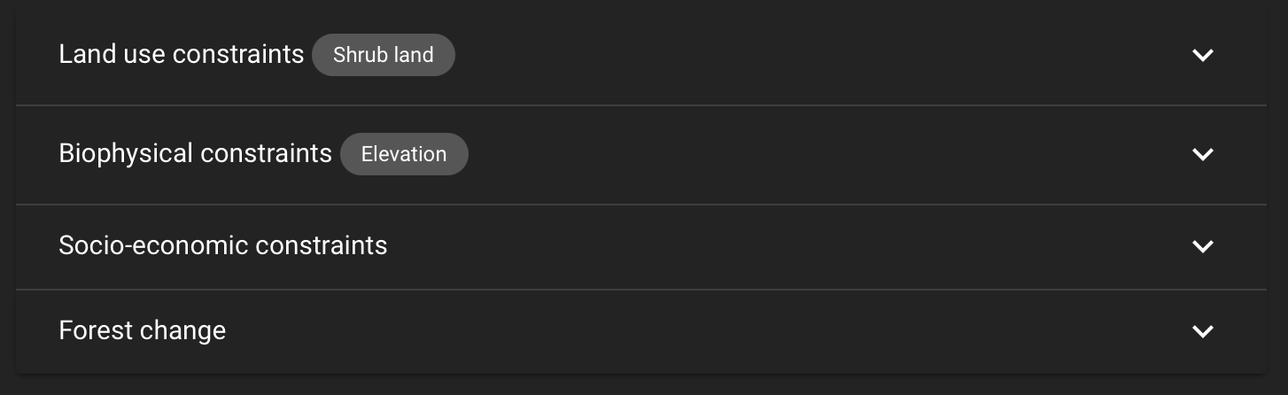
These categories are displayed to the user in expandable panes. Select a category to open its pane and choose the appropriate constraint name in the dropdown menu labeled Criteria. The customization of contraints will appear underneath.
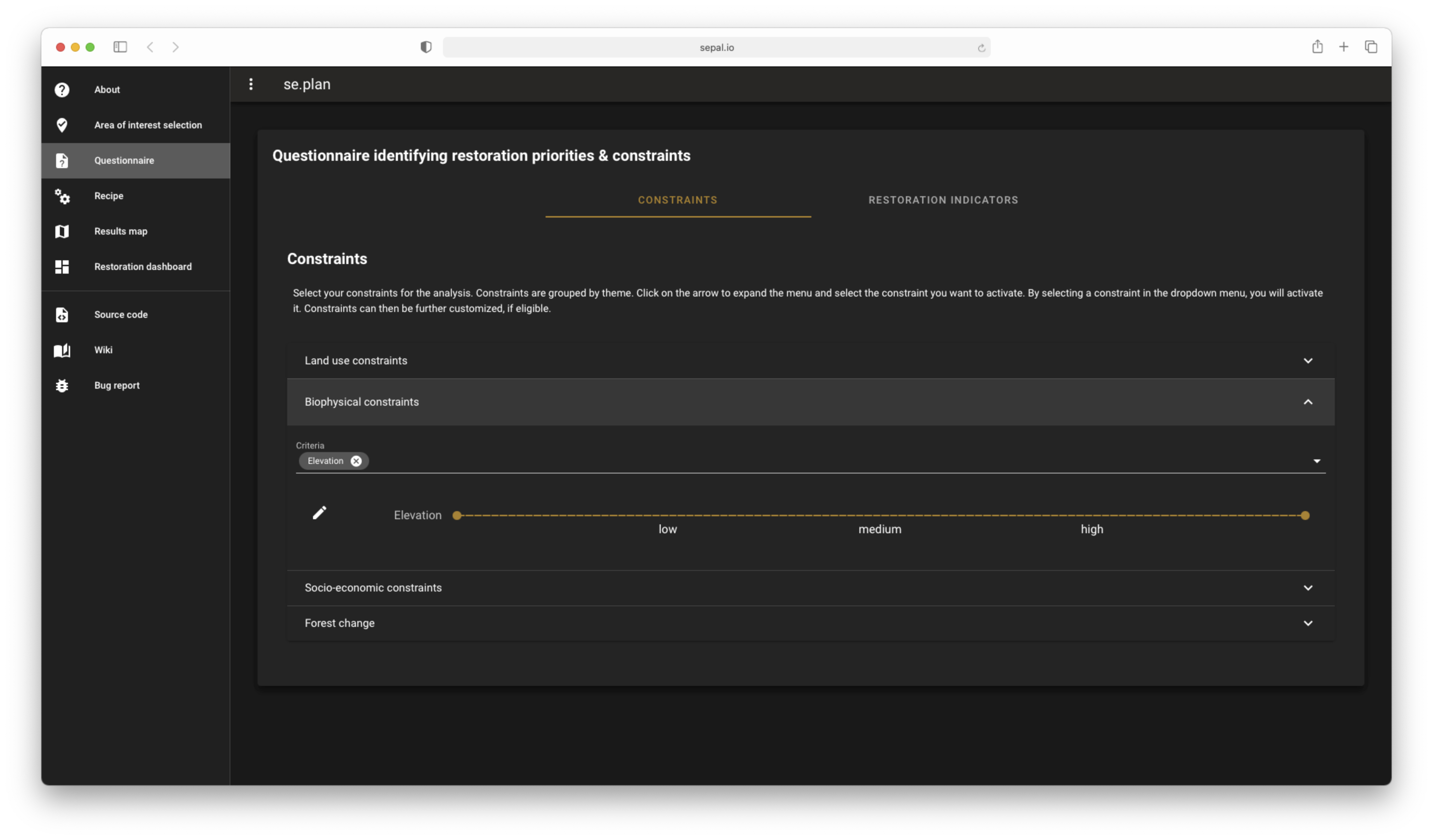
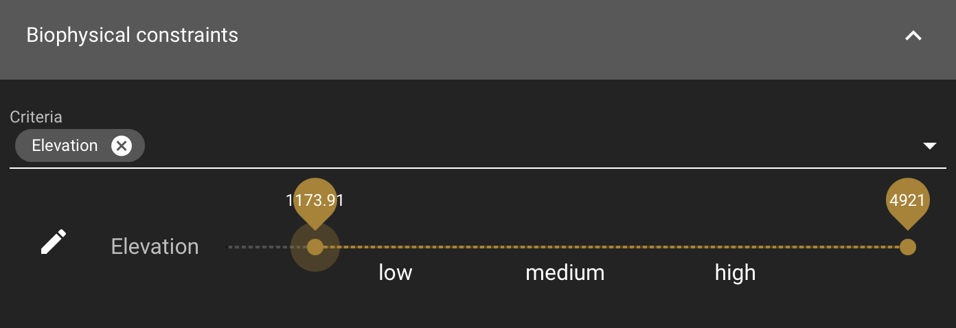
Some constraints are numerical or categorical, for which se.plan enables the user to adjust the values that will be masked from the analysis.
Tip
The values provided in the slider are computed on the fly over your AOI preventing the selection of a filter that would remove all pixels in your area.
Other constraints are binary variables (a value of 1 if a site has the characteristic associated with the variable, or a value of 0 if it does not), which can be set using a switch. For these constraints, users can choose if they want to keep 0s (switch off) or 1s (switch on).
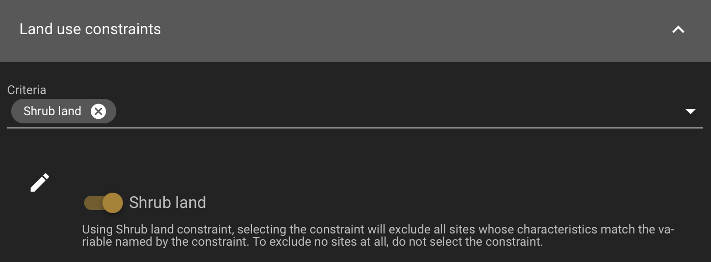
Once the selection is finished, the chosen constraints will be displayed as small chips in the expandable pane title, allowing the user to see all the selected constraints at a glance.
Every selected constraint corresponds to a layer provided by se.plan (listed in the section, Constraints data layers). These layers can be customized in this pane to use national data or to provide information on areas that are not covered by the tool’s default layers. You do not need to add constraints if there aren’t any. In this case, default values will be used and you can simply proceed to the next steps.
Note
To use a customized dataset, it needs to be uploaded as an ee.Image in GEE.
Select the pencil on the left side of the layer name and a pop-up window will appear, which provides:
the layer name as it can be found in GEE;
the unit of the provided layer; and
a map displaying the layer over the AOI using a linear viridis color scale (the legend is in the lower-left corner).
The user can change the layer to any other image from GEE. The map will update automatically to display this new layer and change the legend. If the provided layer uses another unit, please change it. This unit will be used in se.plan’s final report.
Attention
The user needs to have access to the provided custom layer to use it. If the asset cannot be accessed, the application will revert to the default.
Once the modifications are finished, select save to apply the changes to the layer. If the constraint is non-binary, the slider values will be updated to the customized dataset.
Attention
Don’t forget to change the slider values after a layer customization. If your layer uses a different unit, all pixels might be included in your filtering parameters.
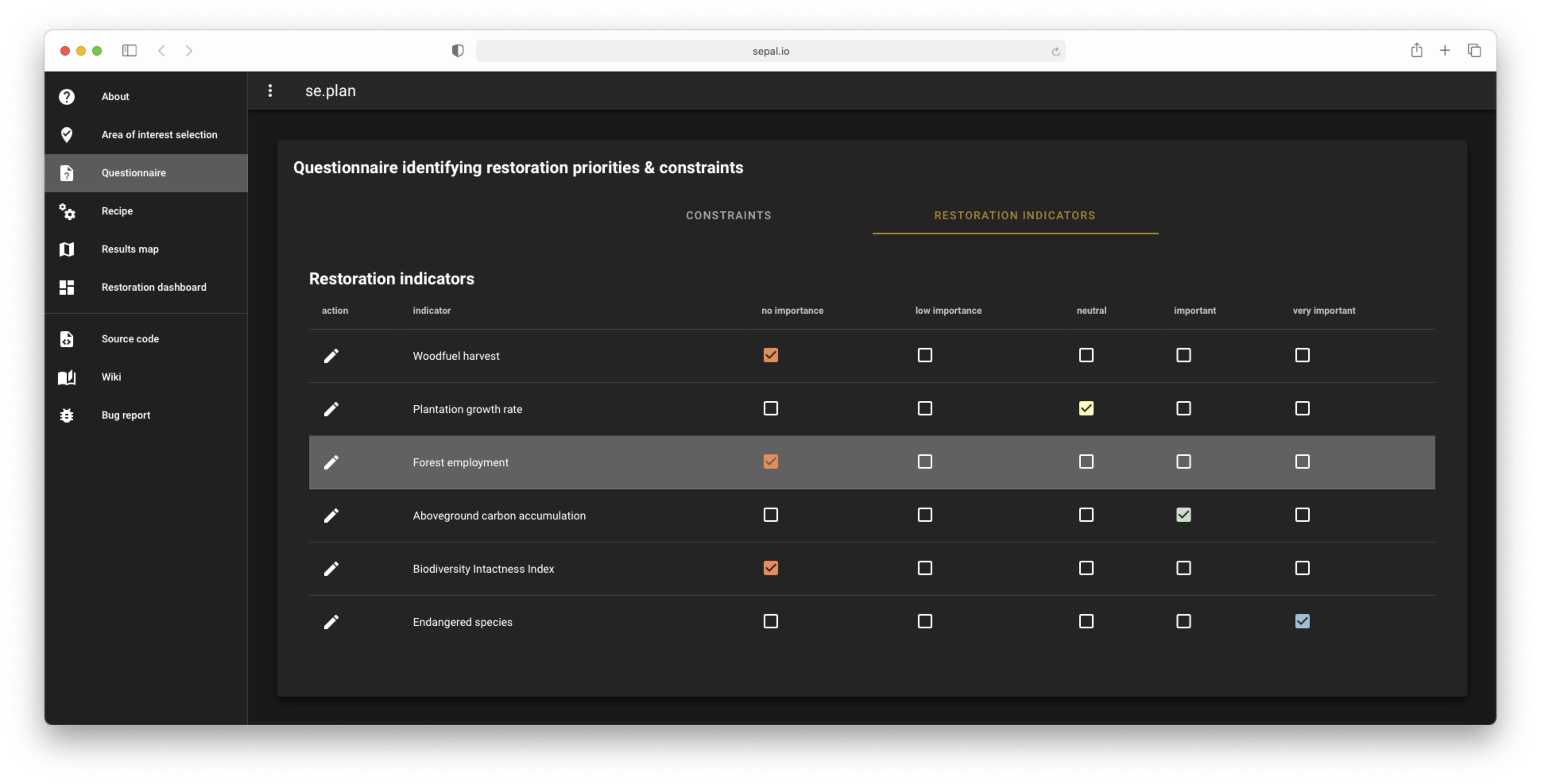
Select indicators#
Users rate the relative importance of benefits from their standpoint (or the standpoint of stakeholders they represent); then, se.plan calculates an Index that indicates each grid cell’s relative restoration value aggregated across all four benefit categories. To rate each indicator, the user simply ticks the corresponding checkbox.
Attention
This step is mandatory if you would like to perform an analysis. If every indicator is set to low (0), then the final output will be 0 everywhere.
Tip
Utilizing the pencil icon next to the indicator name, the user can customize the layer used by se.plan to compute its Index (the editing pop-up pane is the same as the one presented in the previous section).
Select costs#
Users can customize the layers that will be used as Costs in the weighted sum approach by going to the third tab of the questionnaire pane (Costs) and selecting the to open the modification dialog interface (the editing pop-up pane is the same as the one presented in the previous section).

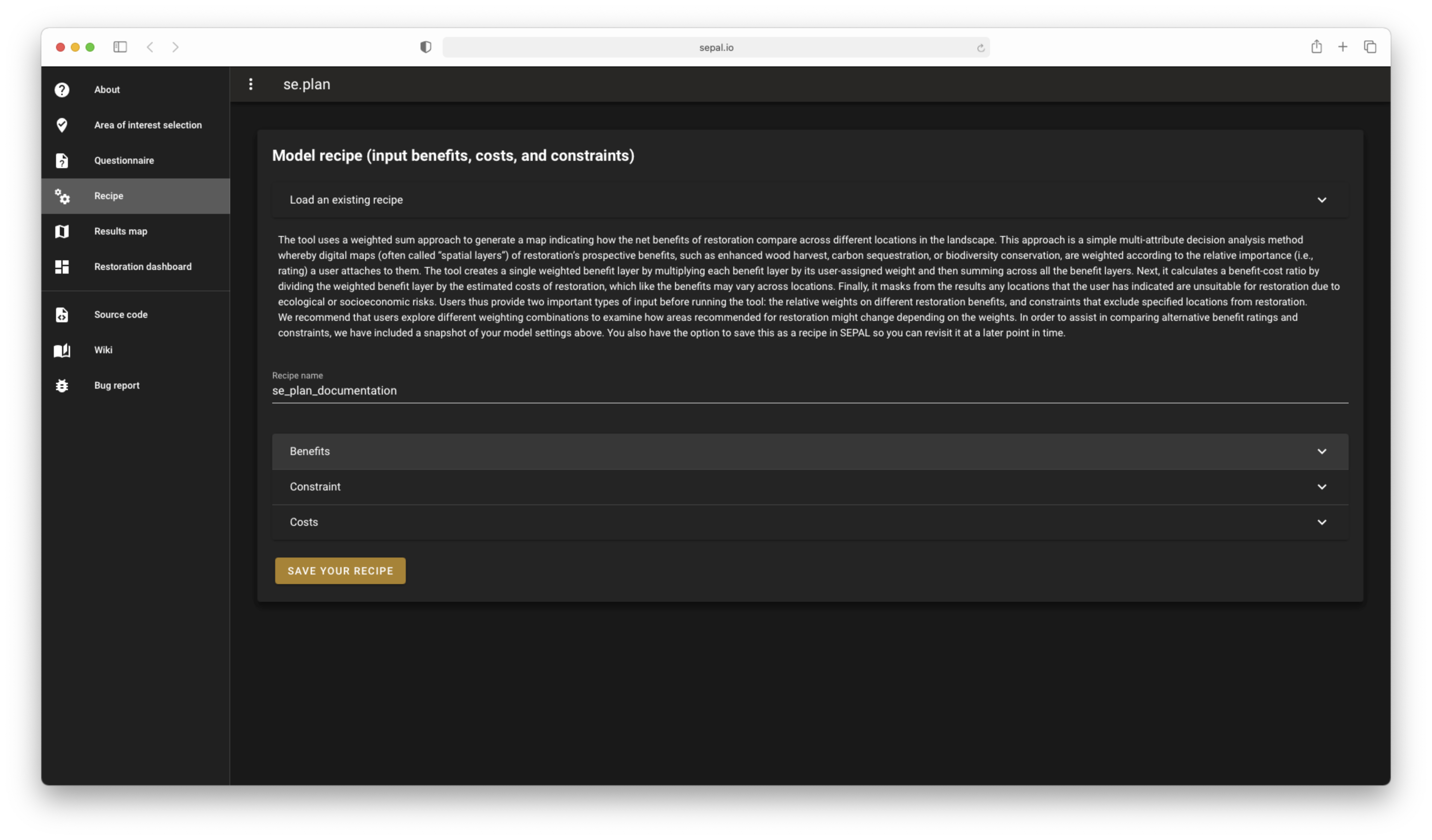
Recipe#
Next, go to the Recipe pane.
Recipe is the base information used by se.plan to compute the Restoration suitability index, which is a .json serialized version of all user-provided inputs in the previous steps that can be shared and reused by other users.
You need to validate your recipe before proceeding to the results. By selecting the Save your recipe button, customization completed in previous steps is recorded and validated.
Validate recipe#
Attention
The AOI and Questionnaire steps need to be completed to validate the recipe.
First, the user should provide a name for the recipe. By default, se.plan uses the current date; however, this can be changed.
Note
If unauthorized folder characters (", `, :code:/, :code: ) are used, they will be automatically replaced by :code:`_.
Once all required inputs are provided, the user can validate the recipe by selecting the validate recipe button.
A .json file will be created in the module_result/restoration_planning_module/ directory of your SEPAL workspace and a summary of your inputs wil be displayed in expandable panes.
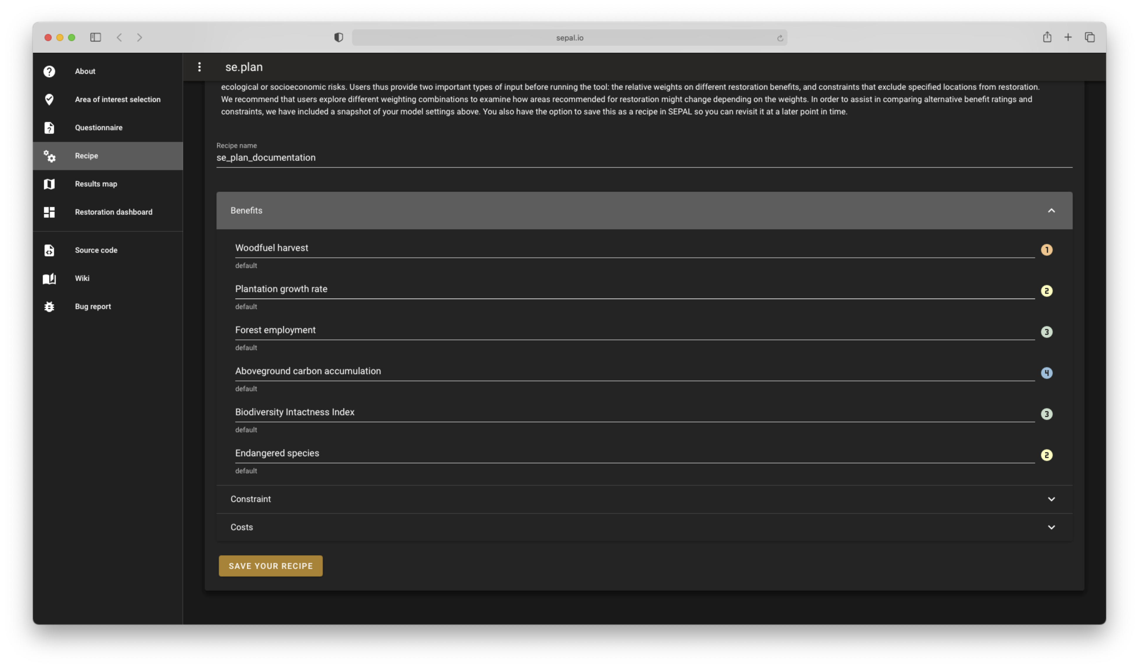
In the Benefits section of the expandable panes, the user will find the list of indicators set in the Questionnaire with the selected weights. If they do not match restoration priorities, they can still be modified in the Questionnaire section.
Note
Don’t forget to validate the recipe every time a change is made in the prior sections (AOI selector and/or Quetionnaire).
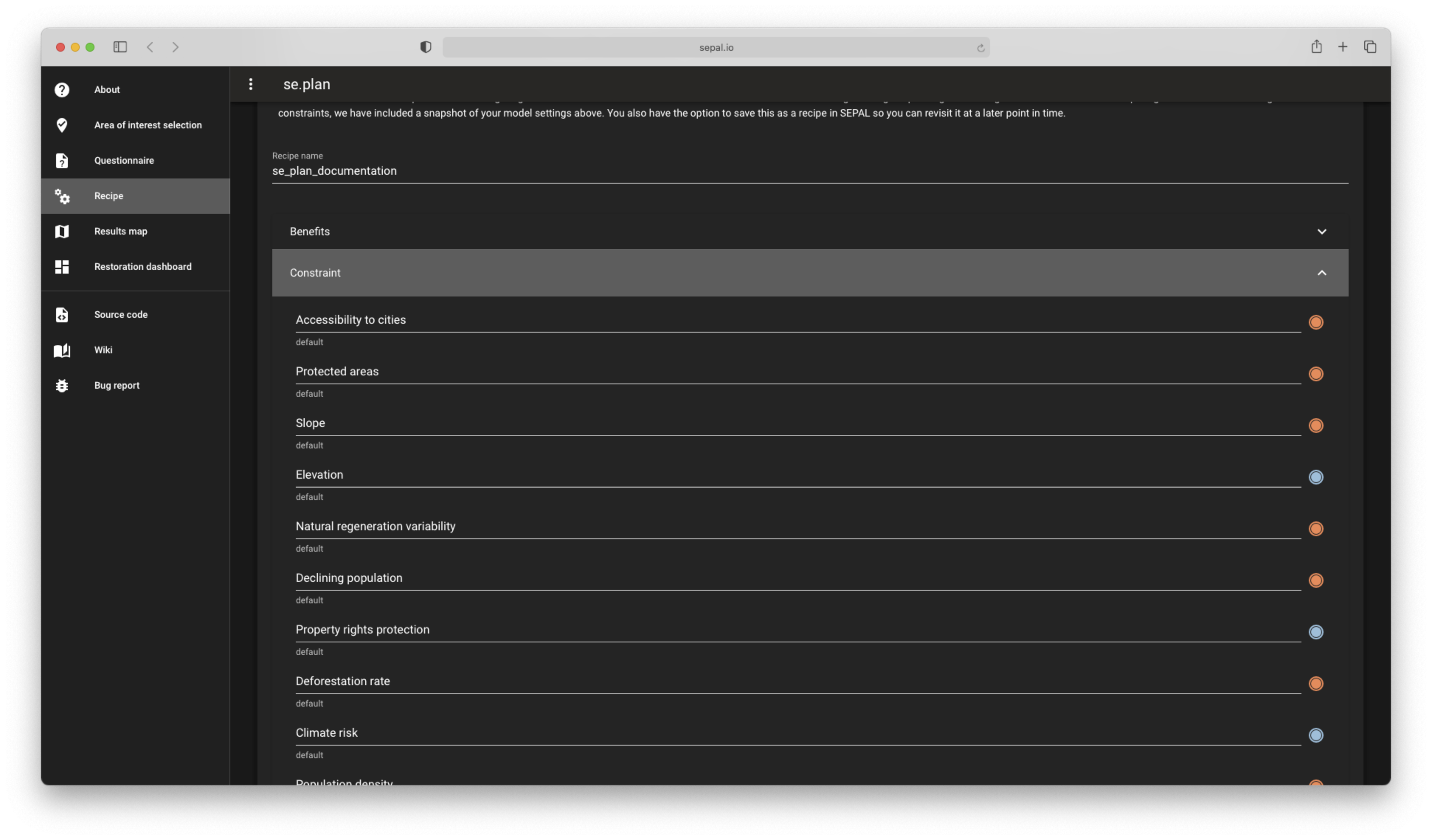
In the Constraints section of the expandable panes, the user will find the complete list of available constraints in the tool. The activated constraint will be displayed in blue; the constraint in red will be ignored in the computation of the Restoration suitability index.
Use existing recipe#
Tip
Loading a recipe can be done without setting any AOI or Questionnaire answers.
The recipe is a simple .json file that is meant to be shared and reused. To do so, use the file selector of the Recipe pane and select a recipe from your SEPAL workspace folder.
Note
Only the
.jsonfiles will be available.If you’ve just uploaded the file, select the
reloadbutton to update the file list.
Tip
By default, the file selector displays the folder where se.plan saves recipes and results. If the user wants to access the rest of their SEPAL workspace, select the parent link in the pop-up menu (on top of the list).
Once the user selects apply the selected recipe, se.plan will reload the AOI specified in the recipe and change all questionnaire answers according to the loaded recipe. It is then automatically validated.

Results map#
Attention
The recipe needs to be validated.
Once the recipe is validated, the compute the restoration map button is released and the Restoration suitability index can be computed. Select the button to view the results map.
The map will be centred on the selected AOI and the value of the Index will be displayed from 1 to 5 using a color-blind, friendly color ramp (red being “not suitable” and blue “very suitable”).
Note
The map can be downloaded as an asset to GEE or as a .tif file. Select the button in the upper-left corner and follow the exportation instructions.
Compute dashboard#
The Compute dashboard button is initially deactivated and will be activated after the Results map correctly returns. Select this button to view the dashboard where results will be displayed (see the section, Restoration dashboard). The dashboard is a report of all restoration information gathered by se.plan during the computation, run from the map and displayed on the Dasboard page.
Select sub-AOI#
The Results from se.plan are given for the initial AOI. Users can also provide sub-AOIs to the tool to provide extra information on smaller areas (the sub-areas are not mandatory to compute the dashboard).
Important
Using sub-AOI is the only way to compare results for different zones, as normalization has been performed on the full extent of the initial AOI.
The sub-AOIs can be selected using a shapefile. The names of the sub-AOIs will be the name set in the selected property.
The sub-AOIs can also be drawn directly on the map. There are three buttons under the cloud icon where you can choose to draw a polygon, rectangle or circle. Select any of them based on your needs. Each time a new geometry is drawn, a pop-up dialogue will ask the user to name it. This name will be used in the final report. You will need to select the Compute dashboard button again to include all sub-AOIs in the report.
Note
The user can still remove some geometry by selecting the button on the map; however, editing is not possible.
Attention
Once the dashboard has been computed, sub-AOIs will be validated (a different color for each); it will be impossible to remove them. New geometries can still be added.

Restoration dashboard#
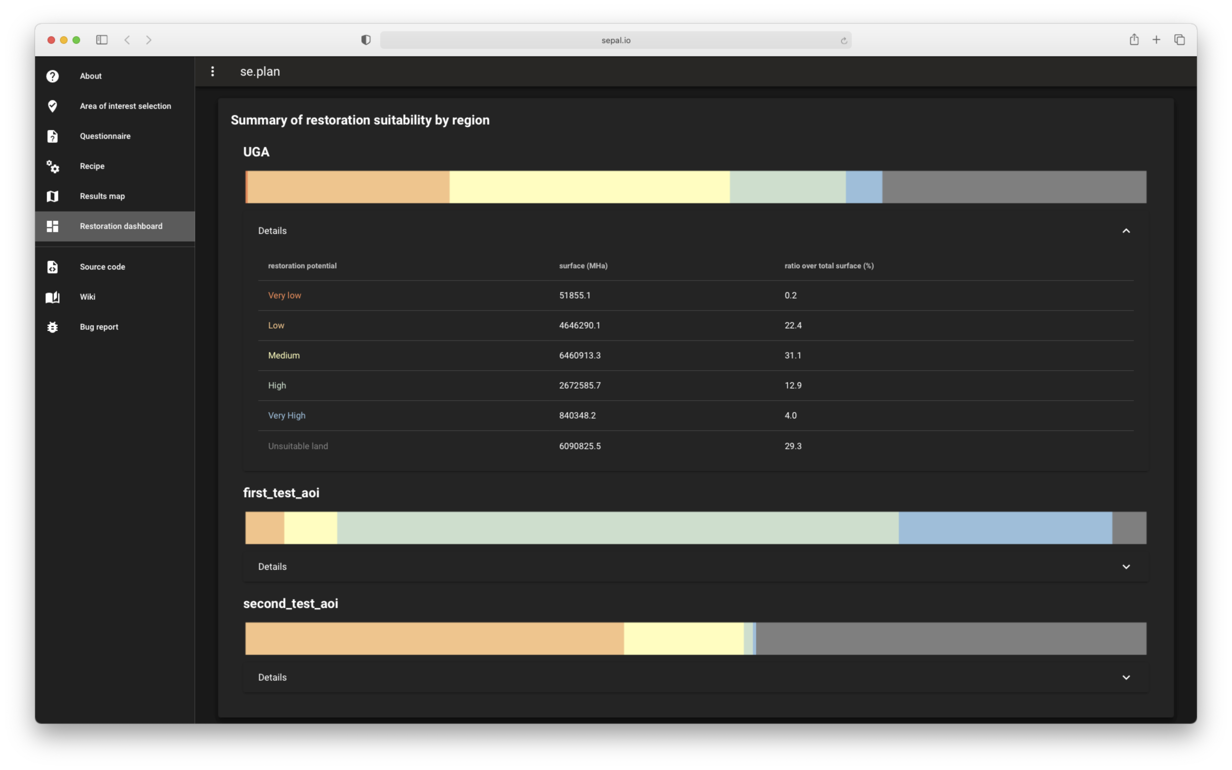
After selecting the compute dashboard button, the report generated from the previous step is displayed in the pane.
Attention
This action can take time, as GEE needs to export and reduce information on the full extent of the user’s initial AOI. Wait until the button stops spinning before changing pages.
The dasboard has two sections:
Summary of restoration suitability by region
AOI - summary by sub-theme
In the first section, the Restoration suitability index is given as proportion of the AOI and the sub-AOIs (note: ISO3 codes are used rather than country names. Select the Details pane to get the surfaces of each restoration value in MHa.
The names used for AOIs are the names selected on the map.
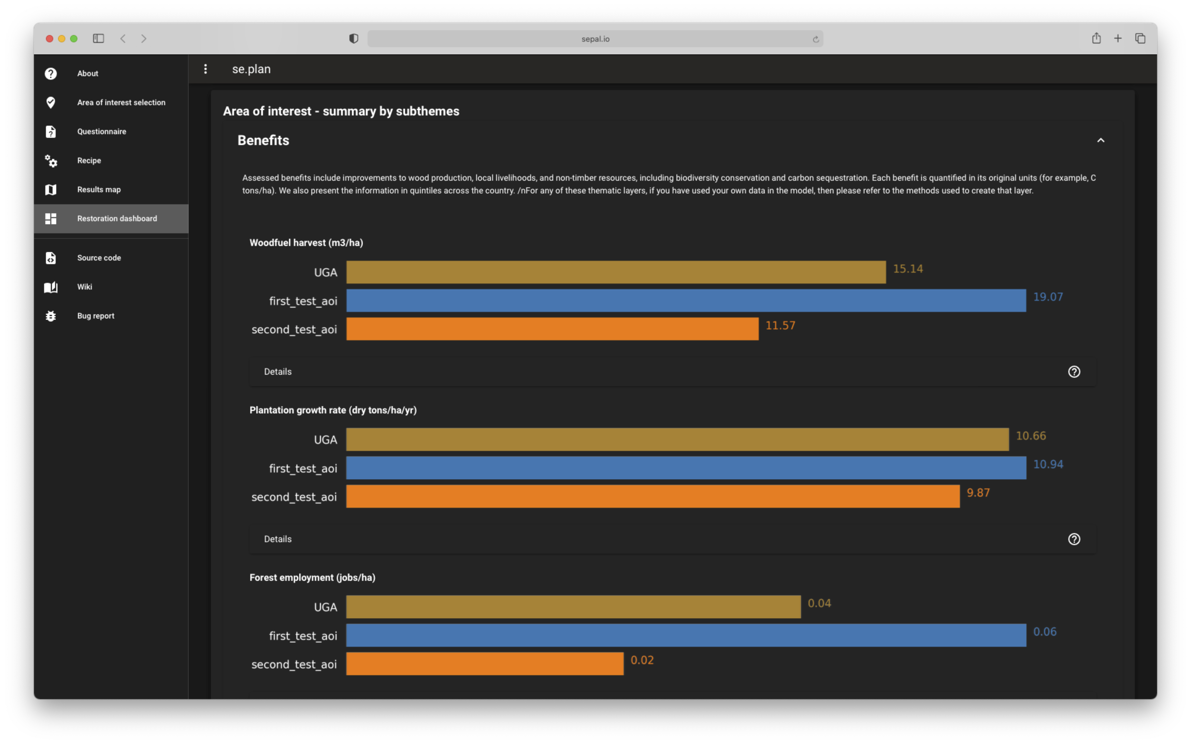
In the second section, the summary is given by sub-theme:
Benefits
The mean value of each benefit is displayed in a bar chart. These charts use the unit corresponding to each layer and display the value for each sub-AOI. Value will be using prefixes from the International System of Units (SI) if the value is not readable in the original unit. The main AOI is first displayed in gold and the sub-AOIs are displayed in the color attributed when the dashboard was computed (i.e. the same as the one used on the map).
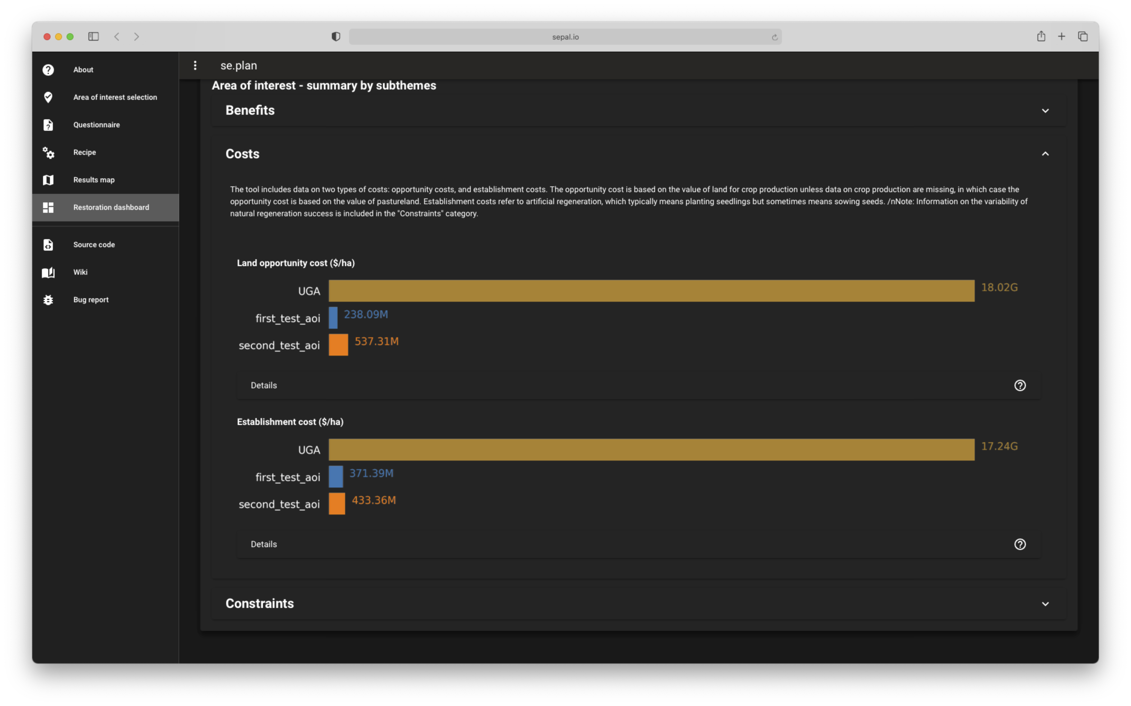
Costs
The sum of each cost over the AOI is displayed in bar charts in the same fashion as the benefits.
Tip
If the surface difference between the main AOI and sub-AOIs is important, as in this example, the total value will also be vastly different.
Constraints
The constraints are displayed in percentages. Each value represents the percentage of surface affected by the filter applied by this constraint over the AOI. Each color represents an AOI (gold for the main AOI and the automatically attributed colors of the sub-AOIs).
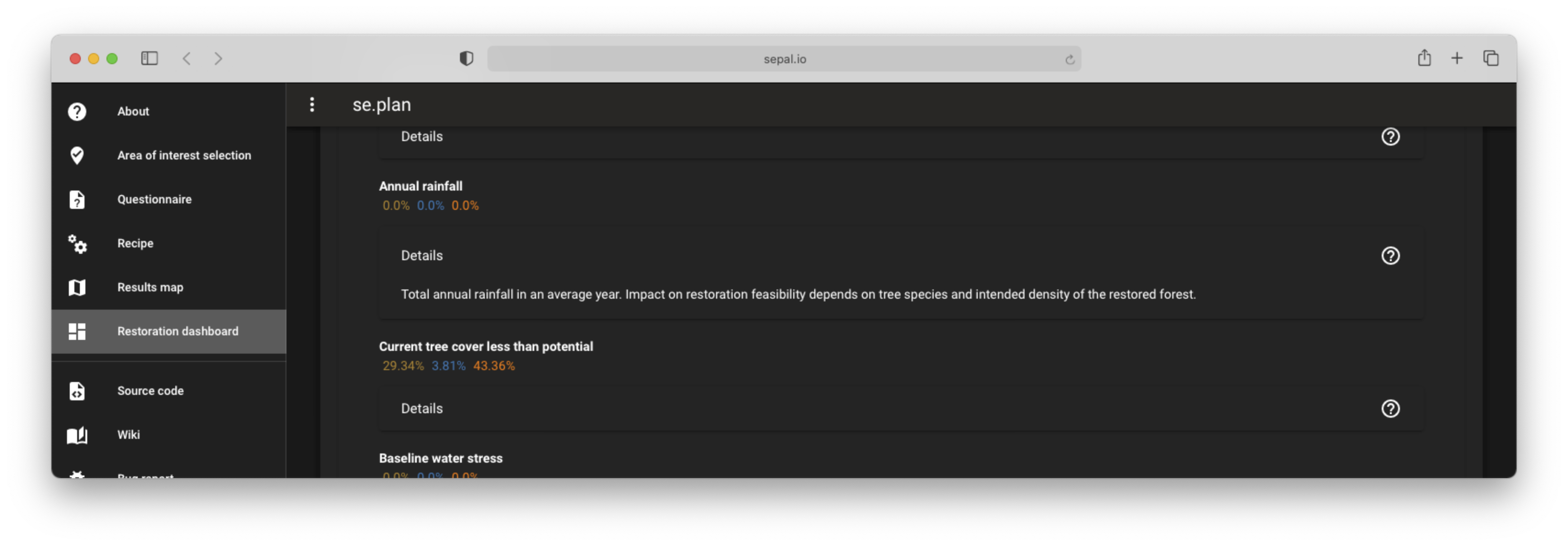
Note
The dashboard is also exported in .csv format to be easily interpreted in any spreadsheet software. It is stored in the same location as the recipe in module_results/se.plan/.
Primary data sources#
The se.plan team obtained data for the default spatial layers in the tool from the following sources.
For determining potential tree cover, data was used from:
Bastin, J.F., Finegold, Y., Garcia, C. et al. 2019. The global tree restoration potential. Science, 365(6448), pp. 76–79. DOI:10.1126/science.aax084
For determining current tree cover, data was used from:
Buchhorn, M., Lesiv, M., Tsendbazar, N.E., Herold, M., Bertels, L. and Smets, B. 2020. Copernicus Global Land Cover Layers—Collection 2. Remote Sensing, 12(108): 1044. doi:10.3390/rs12061044
The team took data for the remaining spatial layers primarily from the sources presented in the following tables (for more information, see Data layers for benefits [benefits], Cost data layers [costs], and Constraints data layers [constraints]).
Costs#
Spatial layer |
Data sources |
|---|---|
Land opportunity cost |
International Food Policy Research Institute. 2019. Global Spatially-Disaggregated Crop Production Statistics Data for 2010 Version 2.0. Harvard Dataverse, V4. https://doi.org/10.7910/DVN/PRFF8V |
FAO (Food and Agriculture Organization of the United Nations). 2020. FAOSTAT: Crops. http://www.fao.org/faostat/en/#data/QC |
|
FAO. 2007. Occurrence of Pasture and Browse (FGGD). https://data.apps.fao.org/map/catalog/srv/eng/catalog.search#/metadata/913e79a0-7591-11db-b9b2-000d939bc5d8 |
|
ESA (European Space Agency). 2017. Land Cover CCI Product User Guide, Version 2. maps.elie.ucl.ac.be/CCI/viewer/download/ESACCI-LC-Ph2-PUGv2_2.0.pdf |
|
FAO. 2018. Gridded Livestock of the World – Latest – 2010 (GLW 3). https://dataverse.harvard.edu/dataverse/glw_3, Harvard Dataverse, V3 |
|
FAO. 2020. FAOSTAT: Livestock Primary. http://www.fao.org/faostat/en/#data/QL |
|
FAO. 2020. RuLIS - Rural Livelihoods Information System. http://www.fao.org/in-action/rural-livelihoods-dataset-rulis/en |
|
World Bank. 2020. World Development Indicators. https://databank.worldbank.org/source/world-development-indicators |
|
CIESIN (Center for International Earth Science Information Network). 2018. Gridded Population of the World, Version 4 (GPWv4): Population Density, Revision 11. NASA Socioeconomic Data and Applications Center (SEDAC). https://doi.org/10.7927/H49C6VHW |
|
Kummu, M., Taka, M. and Guillaume, J. 2018. Gridded global datasets for Gross Domestic Product and Human Development Index over 1990–2015. Scientific Data, 5: 180004. https://doi.org/10.1038/sdata.2018.4 |
|
Establishment cost |
World Bank. n.d. Projects & Operations [project appraisal documents and implementation completion reports for selected projects]. https://projects.worldbank.org/en/projects-operations/projects-home |
Benefits#
Spatial layer |
Sub-theme |
Data sources |
|---|---|---|
Biodiversity intactness index |
Biodiversity conservation |
Newbold, T., Hudson, L., Arnell, A. et al. 2016. Dataset: Global map of the Biodiversity Intactness Index. In: Newbold et al. 2016. Science: Natural History Museum Data Portal (data.nhm.ac.uk). https://doi.org/10.5519/0009936 |
Endangered species |
Biodiversity conservation |
Layer obtained from World Bank, which processed species range maps from: (i) IUCN. The IUCN Red List of Threatened Species. https://www.iucnredlist.org; and (ii) BirdLife International. Data Zone. http://datazone.birdlife.org/species/requestdis |
Unrealized biomass potential |
Carbon sequestration |
Walker, W.S., Gorelik, S.R., Cook-Patton, S.C. et al. 2022. The global potential for increased storage of carbon on land. Proceedings of the National Academy of Sciences, 119(23): e2111312119. https://doi.org/10.1073/pnas.2111312119 |
Forest employment |
Local livelihoods |
Downscaled estimates generated using national data from: International Labour Organization. 2020. Employment by sex and economic activity - ISIC level 2 (thousands). Annual, ILOSTAT database. https://ilostat.ilo.org/data |
Woodfuel harvest |
Local livelihoods |
Downscaled estimates generated using national data from: FAO. 2020. Forestry Production and Trade. In: FAOSTAT. http://www.fao.org/faostat/en/#data/FO |
Plantation growth rate |
Wood production |
Albanito, F., Beringer, T., Corstanje, R. et al. 2016. Carbon implications of converting cropland to bioenergy crops or forest for climate mitigation: a global assessment. GCB Bioenergy, 8: pp. 81–95, https://doi.org/10.1111/gcbb.12242 |
Constraints#
Biophysical#
Spatial layer |
Data sources |
|---|---|
Annual rainfall |
Muñoz Sabater, J. 2019. ERA5-Land monthly averaged data from 1981 to present. Copernicus Climate Change Service (C3S) Climate Data Store (CDS). https://doi.org/10.24381/cds.68d2bb3 |
Baseline water stress |
World Resources Institute. 2021. Aqueduct Global Maps 3.0 Data. https://www.wri.org/data/aqueduct-global-maps-30-data |
Elevation |
Farr, T.G., Rosen, P.A., Caro, E. et al. 2007. The shuttle radar topography mission. Reviews of Geophysics, 45(2): RG2004. https://doi.org/10.1029/2005RG000183 |
Slope |
Farr, T.G., Rosen, P.A., Caro, E. et al. 2007. The shuttle radar topography mission. Reviews of Geophysics, 45(2): RG2004. https://doi.org/10.1029/2005RG000183 |
Terrestrial ecoregion |
FAO. 2012. Global ecological zones for FAO forest reporting: 2010 Update. http://www.fao.org/3/ap861e/ap861e.pdf |
Forest change#
Spatial layer |
Data sources |
|---|---|
Climate risk |
Bastin, J.F., Finegold, Y., Garcia, C. et al. 2019. The global tree restoration potential. Science, 365(6448): pp. 76–79. DOI: 10.1126/science.aax0848; data downloaded from: https://www.research-collection.ethz.ch/handle/20.500.11850/350258 |
Deforestation rate |
ESA. 2017. Land Cover CCI Product User Guide, Version 2. maps.elie.ucl.ac.be/CCI/viewer/download/ESACCI-LC-Ph2-PUGv2_2.0.pdf |
Natural regeneration variability |
Model from Crouzeilles, R., Barros, F.S., Molin, P.G. et al. 2019. A new approach to map landscape variation in forest restoration success in tropical and temperate forest biomes. Journal of Applied Ecology, 56: pp. 2675–2686. https://doi.org/10.1111/1365-2664.13501; applied to data from: ESA. 2017. Land Cover CCI Product User Guide, Version 2. maps.elie.ucl.ac.be/CCI/viewer/download/ESACCI-LC-Ph2-PUGv2_2.0.pdf |
Socioeconomic#
Spatial layer |
Data sources |
|---|---|
Accessibility to cities |
Weiss, D.J., Nelson, A., Gibson, H.S. et al. 2018. A global map of travel time to cities to assess inequalities in accessibility in 2015. Nature. doi:10.1038/nature25181; data downloaded from: https://malariaatlas.org/research-project/accessibility-to-cities |
Country risk premium |
Damodaran, A. 2020. Damodaran Online. http://pages.stern.nyu.edu/~adamodar |
Current land cover |
ESA. 2017. Land Cover CCI Product User Guide, Version 2. maps.elie.ucl.ac.be/CCI/viewer/download/ESACCI-LC-Ph2-PUGv2_2.0.pdf |
Declining population |
CIESIN (Center for International Earth Science Information Network). 2018. Gridded Population of the World, Version 4 (GPWv4): Population Density, Revision 11. NASA Socioeconomic Data and Applications Center (SEDAC). https://doi.org/10.7927/H49C6VHW |
Governance index |
World Bank. 2020. Worldwide Governance Indicators. https://info.worldbank.org/governance/wgi/ |
Land designated for or owned by Indigenous Peoples and local communities (IPLCs) |
Rights and Resources Initiative. 2015. Who Owns the World’s Land? A global baseline of formally recognized indigenous and community land rights. Washington, DC. |
Net imports of forest products |
FAO. 2020. Forestry Production and Trade. In: FAOSTAT. http://www.fao.org/faostat/en/#data/FO |
Population density |
CIESIN (Center for International Earth Science Information Network). 2018. Gridded Population of the World, Version 4 (GPWv4): Population Density, Revision 11. NASA Socioeconomic Data and Applications Center (SEDAC). https://doi.org/10.7927/H49C6VHW |
Perceived property security |
Prindex. 2020. https://www.prindex.net |
Property rights protection |
Downscaled estimates generated using national data from: World Bank. 2020. Worldwide Governance Indicators. https://info.worldbank.org/governance/wgi |
Protected area |
IUCN (International Union for Conservation of Nature). World Database on Protected Areas. https://www.iucn.org/theme/protected-areas/our-work/world-database-protected-areas |
Real interest rate |
World Bank. 2020. World Development Indicators. https://databank.worldbank.org/source/world-development-indicators |
Countries#
Countries and territories in se.plan (organized by World Bank region; ISO refers to the International Organization for Standardization; UNI refers to the Italian National Standards Body; UNDP refers to the United Nations Development Programme; FAOSTAT refers to the Food and Agriculture Organization Corporate Statistical Database; GAUL refers to Global Administrative Unit Layers).
East Asia & Pacific#
Country |
Official name |
ISO3 |
ISO2 |
UNI |
UNDP |
FAOSTAT |
GAUL |
|---|---|---|---|---|---|---|---|
Cambodia |
the Kingdom of Cambodia |
KHM |
KH |
116 |
KHM |
115 |
44 |
China |
the People’s Republic of China |
CHN |
CN |
156 |
CHN |
41 |
147295 |
Cook Islands |
the Cook Islands |
COK |
CK |
184 |
COK |
47 |
60 |
Democratic People’s Republic of Korea |
the Democratic People’s Republic of Korea |
PRK |
KP |
408 |
PRK |
116 |
67 |
Fiji |
the Republic of Fiji |
FJI |
FJ |
242 |
FJI |
66 |
83 |
Indonesia |
the Republic of Indonesia |
IDN |
ID |
360 |
IDN |
101 |
116 |
Kiribati |
the Republic of Kiribati |
KIR |
KI |
296 |
KIR |
83 |
135 |
Lao PDR |
the Lao People’s Democratic Republic |
LAO |
LA |
418 |
LAO |
120 |
139 |
Malaysia |
Malaysia |
MYS |
MY |
458 |
MYS |
131 |
153 |
Marshall Islands |
the Republic of the Marshall Islands |
MHL |
MH |
584 |
MHL |
127 |
157 |
Micronesia |
the Federated States of Micronesia |
FSM |
FM |
583 |
FSM |
145 |
163 |
Mongolia |
Mongolia |
MNG |
MN |
496 |
MNG |
141 |
167 |
Myanmar |
the Republic of the Union of Myanmar |
MMR |
MM |
104 |
MMR |
28 |
171 |
Nauru |
the Republic of Nauru |
NRU |
NR |
520 |
NRU |
148 |
173 |
Palau |
the Republic of Palau |
PLW |
PW |
585 |
PLW |
180 |
189 |
Papua New Guinea |
Independent State of Papua New Guinea |
PNG |
PG |
598 |
PNG |
168 |
192 |
Philippines |
the Republic of the Philippines |
PHL |
PH |
608 |
PHL |
171 |
196 |
Samoa |
the Independent State of Samoa |
WSM |
WS |
882 |
WSM |
244 |
212 |
Solomon Islands |
Solomon Islands |
SLB |
SB |
90 |
SLB |
25 |
225 |
Thailand |
the Kingdom of Thailand |
THA |
TH |
764 |
THA |
216 |
240 |
Timor-Leste |
the Democratic Republic of Timor-Leste |
TLS |
TL |
626 |
TLS |
176 |
242 |
Tokelau |
Tokelau |
TKL |
TK |
772 |
TKL |
218 |
244 |
Tonga |
the Kingdom of Tonga |
TON |
TO |
776 |
TON |
219 |
245 |
Tuvalu |
Tuvalu |
TUV |
TV |
798 |
TUV |
227 |
252 |
Vanuatu |
the Republic of Vanuatu |
VUT |
VU |
548 |
VUT |
155 |
262 |
Viet Nam |
the Socialist Republic of Viet Nam |
VNM |
VN |
704 |
VNM |
237 |
264 |
Central Asia#
Country |
Official name |
ISO3 |
ISO2 |
UNI |
UNDP |
FAOSTAT |
GAUL |
|---|---|---|---|---|---|---|---|
Armenia |
the Republic of Armenia |
ARM |
AM |
51 |
ARM |
1 |
13 |
Azerbaijan |
the Republic of Azerbaijan |
AZE |
AZ |
31 |
AZE |
52 |
19 |
Georgia |
Georgia |
GEO |
GE |
268 |
GEO |
73 |
92 |
Kazakhstan |
the Republic of Kazakhstan |
KAZ |
KZ |
398 |
KAZ |
108 |
132 |
Kyrgyzstan |
the Kyrgyz Republic |
KGZ |
KG |
417 |
KGZ |
113 |
138 |
Tajikistan |
the Republic of Tajikistan |
TJK |
TJ |
762 |
TJK |
208 |
239 |
Turkey |
the Republic of Turkey |
TUR |
TR |
792 |
TUR |
223 |
249 |
Turkmenistan |
Turkmenistan |
TKM |
TM |
795 |
TKM |
213 |
250 |
Uzbekistan |
the Republic of Uzbekistan |
UZB |
UZ |
860 |
UZB |
235 |
261 |
Latin America & Caribbean#
Country |
Official name |
ISO3 |
ISO2 |
UNI |
UNDP |
FAOSTAT |
GAUL |
|---|---|---|---|---|---|---|---|
Antigua and Barbuda |
Antigua and Barbuda |
ATG |
AG |
28 |
ATG |
8 |
11 |
Argentina |
the Argentine Republic |
ARG |
AR |
32 |
ARG |
9 |
12 |
Barbados |
Barbados |
BRB |
BB |
52 |
BRB |
14 |
24 |
Belize |
Belize |
BLZ |
BZ |
84 |
BLZ |
23 |
28 |
Bolivia |
the Plurinational State of Bolivia |
BOL |
BO |
68 |
BOL |
19 |
33 |
Brazil |
the Federative Republic of Brazil |
BRA |
BR |
76 |
BRA |
21 |
37 |
Chile |
the Republic of Chile |
CHL |
CL |
152 |
CHL |
40 |
51 |
Colombia |
the Republic of Colombia |
COL |
CO |
170 |
COL |
44 |
57 |
Costa Rica |
the Republic of Costa Rica |
CRI |
CR |
188 |
CRI |
48 |
61 |
Cuba |
the Republic of Cuba |
CUB |
CU |
192 |
CUB |
49 |
63 |
Dominica |
the Commonwealth of Dominica |
DMA |
DM |
212 |
DMA |
55 |
71 |
Dominican Republic |
the Dominican Republic |
DOM |
DO |
214 |
DOM |
56 |
72 |
Ecuador |
the Republic of Ecuador |
ECU |
EC |
218 |
ECU |
58 |
73 |
El Salvador |
the Republic of El Salvador |
SLV |
SV |
222 |
SLV |
60 |
75 |
French Guiana |
GUF |
86 |
|||||
Grenada |
Grenada |
GRD |
GD |
308 |
GRD |
86 |
99 |
Guatemala |
the Republic of Guatemala |
GTM |
GT |
320 |
GTM |
89 |
103 |
Guyana |
the Co-operative Republic of Guyana |
GUY |
GY |
328 |
GUY |
91 |
107 |
Haiti |
the Republic of Haiti |
HTI |
HT |
332 |
HTI |
93 |
108 |
Honduras |
the Republic of Honduras |
HND |
HN |
340 |
HND |
95 |
111 |
Jamaica |
Jamaica |
JAM |
JM |
388 |
JAM |
109 |
123 |
Mexico |
the United Mexican States |
MEX |
MX |
484 |
MEX |
138 |
162 |
Nicaragua |
the Republic of Nicaragua |
NIC |
NI |
558 |
NIC |
157 |
180 |
Panama |
the Republic of Panama |
PAN |
PA |
591 |
PAN |
166 |
191 |
Paraguay |
the Republic of Paraguay |
PRY |
PY |
600 |
PRY |
169 |
194 |
Peru |
the Republic of Peru |
PER |
PE |
604 |
PER |
170 |
195 |
Saint Kitts and Nevis |
Saint Kitts and Nevis |
KNA |
KN |
659 |
KNA |
188 |
208 |
Saint Lucia |
Saint Lucia |
LCA |
LC |
662 |
LCA |
189 |
209 |
Saint Vincent and the Grenadines |
Saint Vincent and the Grenadines |
VCT |
VC |
670 |
VCT |
191 |
211 |
Suriname |
the Republic of Suriname |
SUR |
SR |
740 |
SUR |
207 |
233 |
Trinidad and Tobago |
the Republic of Trinidad and Tobago |
TTO |
TT |
780 |
TTO |
220 |
246 |
Uruguay |
the Eastern Republic of Uruguay |
URY |
UY |
858 |
URY |
234 |
260 |
Venezuela |
the Bolivarian Republic of Venezuela |
VEN |
VE |
862 |
VEN |
236 |
263 |
Middle East & North Africa#
Country |
Official name |
ISO3 |
ISO2 |
UNI |
UNDP |
FAOSTAT |
GAUL |
|---|---|---|---|---|---|---|---|
Algeria |
the People’s Democratic Republic of Algeria |
DZA |
DZ |
12 |
DZA |
4 |
4 |
Djibouti |
the Republic of Djibouti |
DJI |
DJ |
262 |
DJI |
72 |
70 |
Egypt |
the Arab Republic of Egypt |
EGY |
EG |
818 |
EGY |
59 |
40765 |
Iran |
the Islamic Republic of Iran |
IRN |
IR |
364 |
IRN |
102 |
117 |
Iraq |
the Republic of Iraq |
IRQ |
IQ |
368 |
IRQ |
103 |
118 |
Jordan |
the Hashemite Kingdom of Jordan |
JOR |
JO |
400 |
JOR |
112 |
130 |
Lebanon |
the Lebanese Republic |
LBN |
LB |
422 |
LBN |
121 |
141 |
Libya |
State of Libya |
LBY |
LY |
434 |
LBY |
124 |
145 |
Morocco |
the Kingdom of Morocco |
MAR |
MA |
504 |
MAR |
143 |
169 |
Oman |
the Sultanate of Oman |
OMN |
OM |
512 |
OMN |
221 |
187 |
Palestine |
[Often called West Bank and Gaza] |
PSE |
267 |
||||
Syria |
the Syrian Arab Republic |
SYR |
SY |
760 |
SYR |
212 |
238 |
Tunisia |
the Republic of Tunisia |
TUN |
TN |
788 |
TUN |
222 |
248 |
Western Sahara |
ESH |
268 |
|||||
Yemen |
the Republic of Yemen |
YEM |
YE |
887 |
YEM |
249 |
269 |
South Asia#
Country |
Official name |
ISO3 |
ISO2 |
UNI |
UNDP |
FAOSTAT |
GAUL |
|---|---|---|---|---|---|---|---|
Afghanistan |
the Islamic Republic of Afghanistan |
AFG |
AF |
4 |
AFG |
2 |
1 |
Bangladesh |
the People’s Republic of Bangladesh |
BGD |
BD |
50 |
BGD |
16 |
23 |
Bhutan |
the Kingdom of Bhutan |
BTN |
BT |
64 |
BTN |
18 |
31 |
India |
the Republic of India |
IND |
IN |
356 |
IND |
100 |
115 |
Maldives |
the Republic of Maldives |
MDV |
MV |
462 |
MDV |
132 |
154 |
Nepal |
the Federal Democratic Republic of Nepal |
NPL |
NP |
524 |
NPL |
149 |
175 |
Pakistan |
the Islamic Republic of Pakistan |
PAK |
PK |
586 |
PAK |
165 |
188 |
Sri Lanka |
the Democratic Socialist Republic of Sri Lanka |
LKA |
LK |
144 |
LKA |
38 |
231 |
sub-Saharan Africa#
Country |
Official name |
ISO3 |
ISO2 |
UNI |
UNDP |
FAOSTAT |
GAUL |
|---|---|---|---|---|---|---|---|
Angola |
the Republic of Angola |
AGO |
AO |
24 |
AGO |
7 |
8 |
Benin |
the Republic of Benin |
BEN |
BJ |
204 |
BEN |
53 |
29 |
Botswana |
the Republic of Botswana |
BWA |
BW |
72 |
BWA |
20 |
35 |
Burkina Faso |
Burkina Faso |
BFA |
BF |
854 |
BFA |
233 |
42 |
Burundi |
the Republic of Burundi |
BDI |
BI |
108 |
BDI |
29 |
43 |
Cabo Verde |
Republic of Cabo Verde |
CPV |
CV |
132 |
CPV |
35 |
47 |
Cameroon |
the Republic of Cameroon |
CMR |
CM |
120 |
CMR |
32 |
45 |
Central African Republic |
the Central African Republic |
CAF |
CF |
140 |
CAF |
37 |
49 |
Chad |
the Republic of Chad |
TCD |
TD |
148 |
TCD |
39 |
50 |
Comoros |
the Union of the Comoros |
COM |
KM |
174 |
COM |
45 |
58 |
Congo |
the Republic of the Congo |
COG |
CG |
178 |
COG |
46 |
59 |
Côte d’Ivoire |
the Republic of Côte d’Ivoire |
CIV |
CI |
384 |
CIV |
107 |
66 |
Democratic Republic of the Congo |
the Democratic Republic of the Congo |
COD |
CD |
180 |
COD |
250 |
68 |
Equatorial Guinea |
the Republic of Equatorial Guinea |
GNQ |
GQ |
226 |
GNQ |
61 |
76 |
Eritrea |
the State of Eritrea |
ERI |
ER |
232 |
ERI |
178 |
77 |
Eswatini |
the Kingdom of Eswatini |
SWZ |
SZ |
748 |
SWZ |
209 |
235 |
Ethiopia |
the Federal Democratic Republic of Ethiopia |
ETH |
ET |
231 |
ETH |
238 |
79 |
Gabon |
the Gabonese Republic |
GAB |
GA |
266 |
GAB |
74 |
89 |
Gambia |
the Republic of the Gambia |
GMB |
GM |
270 |
GMB |
75 |
90 |
Ghana |
the Republic of Ghana |
GHA |
GH |
288 |
GHA |
81 |
94 |
Guinea |
the Republic of Guinea |
GIN |
GN |
324 |
GIN |
90 |
106 |
Guinea-Bissau |
the Republic of Guinea-Bissau |
GNB |
GW |
624 |
GNB |
175 |
105 |
Kenya |
the Republic of Kenya |
KEN |
KE |
404 |
KEN |
114 |
133 |
Lesotho |
the Kingdom of Lesotho |
LSO |
LS |
426 |
LSO |
122 |
142 |
Liberia |
the Republic of Liberia |
LBR |
LR |
430 |
LBR |
123 |
144 |
Madagascar |
the Republic of Madagascar |
MDG |
MG |
450 |
MDG |
129 |
150 |
Malawi |
the Republic of Malawi |
MWI |
MW |
454 |
MWI |
130 |
152 |
Mali |
the Republic of Mali |
MLI |
ML |
466 |
MLI |
133 |
155 |
Mauritania |
the Islamic Republic of Mauritania |
MRT |
MR |
478 |
MRT |
136 |
159 |
Mauritius |
the Republic of Mauritius |
MUS |
MU |
480 |
MUS |
137 |
160 |
Mozambique |
the Republic of Mozambique |
MOZ |
MZ |
508 |
MOZ |
144 |
170 |
Namibia |
the Republic of Namibia |
NAM |
NA |
516 |
NAM |
147 |
172 |
Niger |
the Republic of the Niger |
NER |
NE |
562 |
NER |
158 |
181 |
Nigeria |
the Federal Republic of Nigeria |
NGA |
NG |
566 |
NGA |
159 |
182 |
Rwanda |
the Republic of Rwanda |
RWA |
RW |
646 |
RWA |
184 |
205 |
Sao Tome and Principe |
the Democratic Republic of Sao Tome and Principe |
STP |
ST |
678 |
STP |
193 |
214 |
Senegal |
the Republic of Senegal |
SEN |
SN |
686 |
SEN |
195 |
217 |
Seychelles |
the Republic of Seychelles |
SYC |
SC |
690 |
SYC |
196 |
220 |
Sierra Leone |
the Republic of Sierra Leone |
SLE |
SL |
694 |
SLE |
197 |
221 |
Somalia |
the Federal Republic of Somalia |
SOM |
SO |
706 |
SOM |
201 |
226 |
South Africa |
the Republic of South Africa |
ZAF |
ZA |
710 |
ZAF |
202 |
227 |
South Sudan |
the Republic of South Sudan |
SSD |
SS |
728 |
SSD |
277 |
74 |
Sudan |
the Republic of the Sudan |
SDN |
SD |
736 |
SDN |
276 |
6 |
Tanzania |
the United Republic of Tanzania |
TZA |
TZ |
834 |
TZA |
215 |
257 |
Togo |
the Togolese Republic |
TGO |
TG |
768 |
TGO |
217 |
243 |
Uganda |
the Republic of Uganda |
UGA |
UG |
800 |
UGA |
226 |
253 |
Zambia |
the Republic of Zambia |
ZMB |
ZM |
894 |
ZMB |
251 |
270 |
Zimbabwe |
the Republic of Zimbabwe |
ZWE |
ZW |
716 |
ZWE |
181 |
271 |
Data layers for benefits#
Note
Every data layer presented in the following document can be displayed in GEE as an overview of our datasets. Select the provided link in the description to be redirected to the GEE code editor pane. The selected layer will be displayed over Uganda. To modify the country, change the fao_gaul variable Line 7 by your country number (listed in the Country list section in the rightmost column). If you want to export this layer, set the value of to_export (Line 10) and to_drive (Line 13) according to your need.
Hit the run button again to relaunch the computation.
Code used for this display can be found on this page.
In its current form, se.plan provides information on four categories of potential benefits of forest restoration:
biodiversity conservation
carbon sequestration
local livelihoods
wood production
se.plan does not predict the levels of benefits that will occur if forests are restored. Instead, it uses data on benefit-related site characteristics to quantify the potential of a site to provide benefits if it is restored. To clarify this distinction, consider the case of species extinctions. For example, a predictive tool might estimate the number of extinctions avoided if restoration occurs. To do so, it would need to account for restoration scale and interdependencies across sites associated with distances and corridors between restored sites.
se.plan takes a simpler approach: the tool includes information on the total number of critically endangered and endangered amphibians, reptiles, birds and mammals at each site. Sites with a larger number of critically endangered and endangered species have a greater potential number of avoided extinctions. Realizing the benefit of reduced extinctions depends on factors beyond simply restoring an individual site, including the type of forest that is restored (native tree species or introduced tree species, single tree species or multiple tree species, etc.) and the pattern of restoration in the rest of the landscape. Therefore, interpreting se.plan outputs in the context of additional, location-specific information available to a user is important.
Quantitative measures of potential benefits in se.plan should be viewed as averages for a grid cell. Potential benefits could be higher at some locations within a given grid cell and lower at others.
Variable |
Description |
Source |
|---|---|---|
Endangered species (biodiversity conservation) in count |
Total number of critically endangered and endangered amphibians, reptiles, birds and mammals whose ranges overlap a site. Rationale for including in se.plan: sites with a larger number of critically endangered and endangered species are ones where successful forest restoration can potentially contribute to reducing a larger number of extinctions (view in GEE). |
World Bank, which processed over 25 000 species range maps from: (i) IUCN. The IUCN Red List of Threatened Species. https://www.iucnredlist.org; and (ii) BirdLife International. Data Zone. http://datazone.birdlife.org/species/requestdis. Resolution of World Bank layer: 1 km. More information may be found at https://datacatalog.worldbank.org/dataset/terrestrial-biodiversity-indicators; data may be downloaded at http://wbg-terre-biodiv.s3.amazonaws.com/listing.html. See also: (i) Dasgupta, S. and Wheeler, D. 2016. Minimizing Ecological Damage from Road Improvement in Tropical Forests. Policy Research Working Paper: No. 7826. Washington, DC, World Bank; (ii) Danyo, S., Dasgupta, S. and Wheeler, D. 2018. Potential Forest Loss and Biodiversity Risks from Road Improvement in Lao PDR. World Bank Policy Research Working Paper 8569. Washington, DC, World Bank; (iii) Damania, R., Russ, J., Wheeler, D. and Barra, A.F. 2018. The Road to Growth: Measuring the Tradeoffs between Economic Growth and Ecological Destruction, World Development. Elsevier, 101(C): pp. 351–376. |
Biodiversity Intactness Index (BII) gap (Biodiversity conservation) in percent |
The BII describes the average abundance of a large and diverse set of organisms in a given geographical area, relative to the set of originally present species. se.plan subtracts the BII from 100 to measure the gap between full intactness and current intactness. Rationale for including in se.plan: sites with a larger BII gap are ones where successful forest restoration can potentially contribute to reducing a larger gap (view in GEE). |
Newbold, T., Hudson, L., Arnell, A. et al. 2016. Dataset: Global map of the Biodiversity Intactness Index. In: Newbold et al. 2016. Science. Natural History Museum Data Portal (data.nhm.ac.uk). https://doi.org/10.5519/0009936. Resolution of Newbold et al. layer: 1 km; see also: (i) Scholes, R.J. and Biggs, R. 2005. A biodiversity intactness index. Nature, 434(7029): pp.45-49; (ii) Newbold, T., Hudson, L.N., Arnell, A.P., Contu, S., De Palma, A., Ferrier, S., Hill, S.L., Hoskins, A.J., Lysenko, I., Phillips, H.R. and Burton, V.J. 2016. Has land use pushed terrestrial biodiversity beyond the planetary boundary? A global assessment. Science, 353(6296), pp. 288–291. |
Unrealized biomass potential (carbon sequestration) in metric tonnes of carbon (C)/hectare |
Unrealized potential above ground biomass, below ground biomass, and soil organic carbon combined density (mega grammes carbon per hectare) under baseline climate (see below) (view in GEE). |
Walker, W.S., Gorelik, S.R., Cook-Patton, S.C. et al. 2022. The global potential for increased storage of carbon on land. Proceedings of the National Academy of Sciences, 119(23): p. e2111312119. https://doi.org/10.1073/pnas.2111312119. Resolution of Walker et al. layer: 500 m. |
Forest employment (local livelihoods) in count |
Number of forest-related jobs per ha of forest in 2015, combined across three economic activities: forestry, logging and related service activities; manufacture of wood and of products of wood and cork, except furniture; and manufacture of paper and paper products. Varies by country and, when data are sufficient for downscaling, first-level administrative subdivision (e.g. state or province). Rationale for including in se.plan: a higher level of forest employment implies the existence of attractive business conditions for labor-intensive wood harvesting and processing industries, which tends to make forest restoration more feasible when income for local households is a desired benefit. (view in GEE) |
Developed by the se.plan team by downscaling national data from: International Labour Organization. 2020. Employment by sex and economic activity - ISIC level 2 (thousands). Annual, ILOSTAT database. https://ilostat.ilo.org/data |
Woodfuel harvest (local livelihoods) in m<sup>3</sup>/hectare |
Harvest of woodfuel per hectare of forest in 2015. Rationale for including in se.plan: a higher level of woodfuel harvest implies greater demand for woodfuel as an energy source, which tends to make forest restoration more feasible when supply of wood to meet local demands is a desired benefit (view in GEE). |
Developed by se.plan team by downscaling national data from: FAO. 2020. Forestry Production and Trade. In: FAOSTAT. http://www.fao.org/faostat/en/#data/FO |
Plantation growth rate (wood production) in annual dry metric tonnes of woody biomass/hectare |
Potential annual production of woody biomass by fast-growing trees such as eucalypts, poplars and willows. Rationale for including in se.plan: faster growth of plantation trees tends to make forest restoration more feasible when desired benefits include income for landholders and wood supply to meet local and export demands (view in GEE). |
Albanito, F., Beringer, T., Corstanje, R. et al. 2016. Carbon implications of converting cropland to bioenergy crops or forest for climate mitigation: a global assessment. GCB Bioenergy, 8: pp. 81–95, https://doi.org/10.1111/gcbb.12242; resolution of Albanito et al. layer: 55 km. |
Benefit–cost ratio#
In its current form, se.plan includes numerical estimates of four categories of potential restoration benefits for each potential restoration site:
biodiversity conservation
carbon sequestration
local livelihoods
wood production
Denote these benefits, respectively, by \(B_1\), \(B_2\), \(B_3\), and \(B_4\). The data on which the benefit estimates are based have different units. To enable the benefit estimates to be compared with each other, se.plan converts them to the same relative scale, which ranges from 1 (low) to 5 (high). The tool includes two indicators each for \(B_1\) and \(B_3\), and a single indicator for \(B_2\) and \(B_4\). We return to this difference in number of indicators below.
se.plan users rate the relative importance of each benefit on a scale of 1 (low) to 5 (high). The tool treats these ratings as weights and calculates a restoration value index for each site by the weighted-average formula:
Where \(w_1\), \(w_2\), \(w_3\), and \(w_4\) are the user ratings for the four corresponding benefits.
The tool also includes numerical estimates of restoration cost, defined as the sum of opportunity cost and implementation cost expressed in USD per hectare for reference year 2017 for each potential restoration site.
se.plan calculates an approximate benefit–cost ratio by dividing the restoration value index by the estimate of restoration cost:
The benefit-cost ratio in se.plan is approximate in several ways. In particular, the tool does not value potential restoration benefits in monetary terms, and it does not calculate the discounted sum of benefits over a multi-year time period that extends into the future; however, se.plan’s cost estimates account for the future to a greater degree (see Cost data layers). As a final step, the tool converts the benefit–cost ratio across all sites in the user’s AOI to a scale from 1 (low) to 5 (high), reporting this value as the Restoration suitability index on the map and dashboard.
As noted above, se.plan includes two indicators for benefits \(B_1\) (biodiversity conservation) and \(B_3\) (local livelihoods). For \(B_1\), the two indicators are the Biodiversity intactness index and Number of endangered species (denote these two indicators by \(B_1a\) and \(B_1b\)). The tool converts each of these indicators to a 1–5 scale and then calculates the Overall biodiversity benefit, \(B_1\), as their simple average:
se.plan calculates the overall local livelihoods benefit in the same way from its two constituent indicators, Forest employment and Woodfuel harvest.
Cost data layers#
In the case of benefits (Data layers for benefits) and constraints (Constraints data layers), the se.plan team adopted the tool’s data layers primarily from existing sources, with little or no modification of the original layers. In contrast, it developed wholly new data layers for both the opportunity cost and the implementation cost of forest restoration. Developing these layers involved multiple steps, which are described below.
Note
Every data layer presented in the following document can be displayed in GEE as an overview of our datasets. Select the provided link in the description to be redirected to the GEE code editor pane. The selected layer will be displayed over Uganda. To modify the country, change the fao_gaul variable Line 7 to your country number (listed in the Country list section). If you want to export this layer, please set the value of to_export (Line 10) and to_drive (Line 13) according to your need.
Select the run button again to relaunch the computation.
Code used for this display can be found on this page.
Opportunity cost#
Opportunity cost in se.plan refers to the value of land if it is not restored to forest (i.e. the value of land in its current use). A higher opportunity cost tends to make restoration less feasible, although restoration can nevertheless be feasible on land with a high opportunity cost if it generates sufficiently large benefits. se.plan assumes that the alternative land use would be some form of agriculture (either cropland or pastureland). It sets the opportunity cost of potential restoration sites equal to the value of cropland for all sites where crops can be grown, with the opportunity cost for any remaining sites set equal to the value of pastureland.
The value of land in agricultural use is defined as the portion of agricultural profit that is attributable to land as a production input. Economists label this portion “land rent”. Agricultural profit is the difference between the gross revenue a farmer receives from selling agricultural products (= product price × quantity sold) and the expenditures the farmer makes on variable inputs used in production, such as seeds and fertilizer. It is the return earned by fixed inputs, which include labor and capital (e.g. equipment, structures) in addition to land. These relationships imply that the se.plan team needed to sequentially estimate gross revenue, profit and land rent.
Since the se.plan team assumed that forest restoration is intended to be permanent, it estimated land rent in perpetuity: the opportunity cost of forgoing agricultural use of a restored site forever, not just for a single year. The estimates of the long-run opportunity cost in the tool are expressed in USD per hectare for reference year 2017 (view in gee).
Cropland#
The workflow to develop cropland opportunity cost can be summarized as follows:
The se.plan team obtained gridded data on 2010 value of crop production per hectare (i.e. gross revenue per hectare) from the International Food Policy Research Institute’s MapSPAM project (International Food Policy Research Institute, 2019; Yu et al., 2020). The resolution of this layer was 5 arc-minutes (approximately 10 km at the equator).
The team updated the MapSPAM data to 2017 using country-specific data on total cereal yield from FAOSTAT (FAO, 2020a) and the global producer price index for total cereals (also from FAOSTAT). The MapSPAM data reflect gross revenue from a much wider range of crops than cereals, but cereals are the dominant crops in most countries.
The team multiplied the data from Step 2 by an estimate of the share of crop revenue that was attributable to land (i.e. the land-rent share). The rent-share estimates differed across countries and, where data permitted, by first-level administrative subdivisions (e.g. states, provinces) within countries. The team developed the rent-share estimates through a two-step procedure: #. It used 229 859 annual survey observations spanning 2004–2017 from 196 327 unique farm households (FAO, 2020c) in 32 LMICs to statistically estimate a model that related profit from growing crops to fixed inputs. Table E1 shows the distribution of observations by country in the statistical model, and Table E2 shows the estimation results for the model. The dependent variable in the model was the natural logarithm of profit (“lnQuasiRent” in the table), and fixed inputs were represented by the natural logarithms of cultivated area (“lncultivated”) and family labor (“lnfamlabor”); a binary (“dummy”) variable indicated whether the farm was mechanized (“dmechuse”). The model also included year dummies and fixed effects for regions (countries or first-level subdivisions, depending on the survey), which controlled for unobserved factors that varied across time but not regions (the year dummies) and unobserved factors that varied across regions but not time (region-fixed effects). Post-estimation, the team calculated land rent for each observation by multiplying profit by 0.325, the estimated coefficient on the log cultivated area variable. This procedure assumes that the coefficients on inputs in the log–log profit model can be interpreted as profit shares. This assumption is valid if production has constant returns to scale (i.e. if the coefficients add up to 1, which they approximately do in the model). #. The team used sampling weights from the surveys to calculate mean values of crop revenue and land rent for each region in the sample. It then calculated the ratio of mean land rent to mean crop revenue (i.e. the land-rent share for each region); it also statistically related the rent shares to a set of spatial variables, which included: the region’s gross domestic product (GDP) per capita in 2015 (Kummu et al., 2018); its population density in 2015 (CIESIN, 2018); the strength of property rights in it (see discussion of this variable in Appendix F); area shares of terrestrial ecoregions in it (Olson and Dinerstein, 2002); and its classification by World Bank region. Table E3 shows the estimation results for the rent-share model. The team used this model to predict rent shares for the LMICs spanned by se.plan and, where possible, first-level subdivisions within them.
The team estimated the value of cropland in perpetuity by dividing the annual land rent estimates from Step 3 by 0.07, under the assumption that the financial discount rate is 7 percent. It based this assumption on the mean value of real interest rates across the LMICs in the tool (World Bank, 2020).
Pastureland#
The se.plan team used similar procedures to estimate the value of pastureland. In place of cropland in Step 1 and Step 2, it:
Predicted pastureland area in 2015 by first statistically relating pastureland percentage in 2000 (FAO, 2007; Van Velthuizen et al., 2007) to a set of land cover variables for 2000 at 300 m resolution from the European Space Agency (ESA, 2017), then using the resulting statistical model and 2015 values of the land cover variables to predict 2015 pastureland area within each 300 m grid cell.
Calculated gross revenue from livestock around 2017 by multiplying gridded data on livestock numbers (buffaloes, cattle, goats, horses and sheep) in 2010 at 10 km resolution (FAO, 2018) by 2017 estimates of production value per animal, calculated by using country-specific data on stocks of animals and production value of livestock products from FAOSTAT (FAO, 2020b). It adjusted the resulting estimates of gross revenue per grid cell to include production only from grazing lands, not from feedlots, by using FAO estimates of national shares of meat production from grazing lands provided by the World Bank.
Calculated gross revenue per hectare around 2017 by dividing gross revenue from Step 2 by pastureland area from Step 1.
Compared to cropland in Step 3, household survey data on livestock production on pastureland (FAO, 2020c) were too limited to estimate land-rent shares that varied across countries or first-level subdivisions. Instead, the statistical rent-share estimate used in the tool (6.1 percent of gross revenue) is identical across all countries and first-level subdivisions. Step 4 was the same as for cropland.
Implementation costs#
Implementation costs refer to the expense of activities required to regenerate forests. They include both:
initial expenses incurred in the first year of restoration (establishment costs), which are associated with such activities as site preparation, planting and fencing; and
expenses associated with monitoring, protection, and other activities in years following establishment (operating costs), which are required to enable the regenerated stand to reach the “free to grow” stage.
se.plan does not report these two components of implementation costs separately. Instead, it reports the aggregate cost of restoring a site (in USD per hectare for reference year 2017) by adding up the estimates of opportunity costs and implementation costs. This aggregate cost is the cost variable that it includes in the benefit–cost ratio (Appendix D). The estimates of implementation costs vary by country and, for countries with sufficient data, by first-level subdivision.
As previously discussed, se.plan assumes that current land use is some form of agriculture. It therefore also assumes that regeneration requires planting, as sources of propagules for natural regeneration are often not adequate on land that has been cleared for agriculture. However, the tool does not ignore natural regeneration as a restoration option, as it includes a constraint layer that predicts the variability of natural regeneration success (see Cost data layers; view in GEE).
The se.plan team estimated implementation costs in three steps:
The team extracted data on implementation costs from project appraisal reports and implementation completion reports for 50 World Bank afforestation and reforestation projects spanning 24 LMICs during the past two to three decades. Afforestation refers to regeneration of sites where the most recent land use was not forest (e.g. agriculture), while reforestation refers to regeneration of sites that only recently lost their forest cover (e.g. due to harvesting or wildfire). Whenever possible, the team extracted data on operating costs in addition to data on establishment costs, with operating costs typically extending up to three to five years after establishment (depending on project and site). It converted all estimates to a per-hectare basis, expressed in constant 2011 USD. It classified the estimates by country and, where possible, first-level subdivision.
The team statistically related the natural logarithm of implementation cost per hectare to a set of variables hypothesized to explain it, including: (i) GDP per capita, also natural log transformed (Kummu et al., 2018); (ii) a dummy variable distinguishing reforestation from afforestation (regeneration of sites where the most recent land use was not forest [e.g. agriculture]); (iii) a dummy variable distinguishing natural regeneration from planting; (iv) the total regenerated area (natural log transformed); (v) dummy variables giving the dominant biome in the region (tropical or subtropical, versus temperate/boreal; (FAO, 2013); (vi) a dummy variable indicating whether the project began pre- or post-2010; (vii) a dummy variable that can be interpreted as indicating whether the cost estimate accounted for project overhead costs or not (“UnitArea”); and (viii) a set of dummy variables that indicated projects that included special types of regeneration that did not commonly occur in the dataset, which mainly referred to regeneration of small to large stands of trees on interior sites (Table E4 shows estimation results for the model).
The team predicted spatial estimates of implementation costs by region (country or first-level subdivision) by inserting into the model: gridded GDP estimates for 2011; the mean of project area in the estimation sample; and the biome variables. All other binary variables were set to 0. As a final step, the team converted the predicted implementation costs to constant 2017 USD using annual inflation rates between 2012 and 2017.
References#
CIESIN (Center for International Earth Science Information Network). 2018. Gridded Population of the World, Version 4 (GPWv4): Population Density, Revision 11. NASA Socioeconomic Data and Applications Center (SEDAC). https://doi.org/10.7927/H49C6VHW
ESA (European Space Agency). 2017. Land Cover CCI Product User Guide, Version2. maps.elie.ucl.ac.be/CCI/viewer/download/ESACCI-LC-Ph2-PUGv2_2.0.pdf
IFPRI (International Food Policy Research Institute). 2019. Global Spatially-Disaggregated Crop Production Statistics Data for 2010 Version 2.0. Harvard Dataverse, V4. https://doi.org/10.7910/DVN/PRFF8V
Kummu, M., Taka, M. and Guillaume, J. 2018. Gridded global datasets for Gross Domestic Product and Human Development Index over 1990–2015. Scientific Data, 5: 180004. https://doi.org/10.1038/sdata.2018.4
Olson, D.M., and Dinerstein, E. 2002. The Global 200: Priority ecoregions for global conservation. Annals of the Missouri Botanical Garden, 89: 125–126. https://geospatial.tnc.org/datasets/7b7fb9d945544d41b3e7a91494c42930_0
Van Velthuizen, H., Huddleston, B., Fischer, G., Salvatore, M., Ataman, E. et al. 2007. Mapping biophysical factors that influence agricultural production and rural vulnerability. Environment and Natural Resources Series No. 11. Rome, FAO.
Yu, Q., You, L., Wood-Sichra, U., Ru, Y., Joglekar, A.K.B. et al. 2020. A cultivated planet in 2010: Part 2 – The global gridded agricultural production maps. Earth System Science Data. https://doi.org/10.5194/essd-2020-11
FAO. 2007. Occurrence of Pasture and Browse (FGGD). https://data.apps.fao.org/map/catalog/srv/eng/catalog.search#/metadata/913e79a0-7591-11db-b9b2-000d939bc5d8
FAO. 2013. Global Ecological Zones (second edition). https://data.apps.fao.org/map/catalog/srv/eng/catalog.search#/metadata/2fb209d0-fd34-4e5e-a3d8-a13c241eb61b
FAO. 2018. Gridded Livestock of the World – Latest – 2010 (GLW 3). https://dataverse.harvard.edu/dataverse/glw_3, Harvard Dataverse, V3.
FAO. 2020a. FAOSTAT: Crops. http://www.fao.org/faostat/en/#data/QC
FAO. 2020b. FAOSTAT: Livestock Primary. http://www.fao.org/faostat/en/#data/QL
FAO. 2020c. RuLIS - Rural Livelihoods Information System. http://www.fao.org/in-action/rural-livelihoods-dataset-rulis/en
World Bank. 2020. World Development Indicators. https://databank.worldbank.org/source/world-development-indicators
World Bank. n.d. Projects & Operations. Project appraisal documents and implementation completion reports for selected projects. https://projects.worldbank.org/en/projects-operations/projects-home
Constraints data layers#
se.plan includes various constraints that enable users to restrict restoration to sites that satisfy specific criteria. Many of the constraints can be viewed as indicators of risk, which allows users to avoid sites where the risk of failure or undesirable impacts might be unacceptable. Values of the constraints should be viewed as average values for a site, with some locations within a site likely having higher or lower values. The constraints are grouped into four categories: biophysical; current land cover; forest change; and socioeconomic.
Note
Every data layer presented in the following document can be displayed in GEE as an overview of our datasets. Select the provided link in the description to be redirected to the GEE code editor pane. The selected layer will be displayed over Uganda. To modify the country, change the fao_gaul variable Line 7 to your country number (listed in the Country list* section). If you want to export this layer, please set the value of to_export (Line 10) and to_drive (Line 13), according to your need.
Select the run button again to relaunch the computation.
Code used for this display can be found on this page.
Potential constraint#
Attention
This contraint is hard-coded in the tool; the user cannot customize it. It covers the entire world, meaning that it will not mask all of your analysis if se.plan is run outside of the LMIC.
Variable |
Units/measure |
Description |
Source |
|---|---|---|---|
Potential for restoration |
Binary |
Sites that have the potential for restoration. Their tree-cover fraction is less than its potential and they are not in urban areas (view in GEE). |
Bastin, J.-F. & Finegold, Y., Garcia, C., Mollicone, D., Rezende, M., Routh, D., Zohner, C. and Crowther, T. 2019. The global tree restoration potential. Science, 365: 76-79. https://doi.org/10.1126/science.aax0848 Buchhorn, M., Lesiv, M., Tsendbazar, N.-E., Herold, .M, Bertels, L. and Smets, B. 2020. Copernicus Global Land Cover Layers—Collection 2. Remote Sensing, 12(6): 1044. https://doi.org/10.3390/rs12061044 |
Biophysical constraints#
Variable |
Units/measure |
Description |
Source |
|---|---|---|---|
Elevation |
Metres |
Void-filled digital elevation dataset from Shuttle Radar Topography Mission (SRTM) (view in GEE). |
Farr, T.G., Rosen, P.A., Caro, E. et al. 2007. The shuttle radar topography mission: Reviews of Geophysics, 45(2): RG2004. https://doi.org/10.1029/2005RG000183 |
Slope |
Degrees |
The elevation dataset was used to calculate slope in units of degrees from horizontal, with greater values indicating steeper inclines (view in GEE). |
Farr, T.G., Rosen, P.G., Caro, E. et al. 2007. The shuttle radar topography mission. Reviews of Geophysics, 45(2): RG2004. https://doi.org/10.1029/2005RG000183 |
Annual rainfall |
MM/YR |
High-resolution estimates of total annual rainfall based on mean value from past 30 year measurements (view in gee). |
Muñoz Sabater, J. 2019. ERA5-Land monthly averaged data from 1981 to present. Copernicus Climate Change Service (C3S) Climate Data Store (CDS). https://doi.org/10.24381/cds.68d2bb3 |
Baseline water stress |
Scale (0 to 5) |
Ratio of total water withdrawals (for consumptive and non-consumptive domestic, industrial, irrigation and livestock uses) to available renewable supplies of surface water and groundwater, averaged across months of the year and converted to a numerical scale. Higher values of the scale indicate greater water stress (view in GEE). |
World Resources Institute. 2021. Aqueduct Global Maps 3.0 Data. https://www.wri.org/data/aqueduct-global-maps-30-data |
Current land cover#
Variable |
Units/measure |
Description |
Source |
|---|---|---|---|
Terrestrial ecoregion |
Ecological zone labels |
Classification of Earth’s land surface into 20 ecological zones, which have relatively homogeneous vegetation formations under natural conditions and similar physical features (e.g. climate) (view in GEE). |
FAO. 2012. Global ecological zones for fao forest reporting: 2010 Update. http://www.fao.org/3/ap861e/ap861e.pdf |
Forest change constraints#
Variable |
Units/measure |
Description |
Source |
|---|---|---|---|
Deforestation rate |
Percent/YR |
Annual rate of tree-cover loss within a 5 km buffer around a site during 2005–2015, expressed as a positive percentage of total tree cover. Higher values indicate higher rates of loss. The value is zero in areas without deforestation (i.e. areas with expanding tree cover) (view in GEE). |
Developed by the se.plan team, using data from: ESA. 2017, Land Cover CCI Product User Guide, Version 2. maps.elie.ucl.ac.be/CCI/viewer/download/ESACCI-LC-Ph2-PUGv2_2.0.pdf |
Climate risk |
Percentange of area |
Difference between potential tree cover in 2050 if climate trends continue, and potential tree cover under current climatic conditions. Positive values indicate increases in potential tree cover, while negative values indicate decreases (view in GEE). |
Bastin, J.F., Finegold, Y., Garcia, C. et al. 2019. The global tree restoration potential. Science, 365(6448): pp. 76–79. DOI: 10.1126/science.aax0848; data downloaded from: https://www.research-collection.ethz.ch/handle/20.500.11850/350258 |
Natural regeneration variability |
Scale (0 to 1) |
Measure of variability of forest restoration in fostering recovery of biodiversity to typical levels in natural native forests. Higher values indicate that biodiversity recovery is more variable (i.e. less predictable) (view in GEE). |
Developed by the se.plan team, using model from: Crouzeilles, R., Barros, F.S., Molin, P.G. et al. 2019. A new approach to map landscape variation in forest restoration success in tropical and temperate forest biomes. Journal of Applied Ecolology, 56: pp. 2675– 2686. https://doi.org/10.1111/1365-2664.13501; and data from: ESA. 2017. Land Cover CCI Product User Guide, Version 2. maps.elie.ucl.ac.be/CCI/viewer/download/ESACCI-LC-Ph2-PUGv2_2.0.pdf |
Socioeconomic constraints#
Variable |
Units/measure |
Description |
Source |
|---|---|---|---|
Protected areas |
Binary (0 or 1) |
Value of 1 indicates that a site is located in a protected area; value of 0 indicates it is not (view in GEE). |
IUCN (International Union for Conservation of Nature). World Database on Protected Areas. https://www.iucn.org/theme/protected-areas/our-work/world-database-protected-areas |
Population density |
Persons per km<sup>2</sup> |
Modelled distribution of human population for 2020, based on census data for the most disaggregated administrative units available (view in GEE). |
CIESIN (Center for International Earth Science Information Network). 2018. Gridded Population of the World, Version 4 (GPWv4): Population Density, Revision 11. NASA Socioeconomic Data and Applications Center (SEDAC). https://doi.org/10.7927/H49C6VHW |
Declining population |
Binary (0 or 1) |
Value of 1 indicates that human population in a 5 km buffer around a site declined during 2010–2020; value of 0 indicates it rose or did not change (view in GEE). |
Developed by the se.plan team, using 2.5 arc-minute data from: CIESIN (Center for International Earth Science Information Network). 2018. Gridded Population of the World, Version 4 (GPWv4): Population Density, Revision 11. NASA Socioeconomic Data and Applications Center (SEDAC). https://doi.org/10.7927/H49C6VHW |
Property rights protection |
Index (−2.5 to +2.5) |
Downscaled version of the World Bank’s Rule of Law Governance Indicator, which is often interpreted as an indicator of property rights protection. Values range from −2.5 (very weak property rights) to +2.5 (very strong property rights). Varies by country and, when data are sufficient for downscaling, first-level administrative subdivision (e.g. state or province) (view in GEE). |
Developed by the se.plan team by downscaling national data from: World Bank. 2020. Worldwide Governance Indicators. https://info.worldbank.org/governance/wgi/ |
Accessibility to cities |
Minutes |
Travel time from a site to the nearest city in 2015 (view in GEE). |
Weiss, D.J., Nelson, A., Gibson, H.S. et al. 2018. A global map of travel time to cities to assess inequalities in accessibility in 2015. Nature. doi:10.1038/nature25181; data downloaded from: https://malariaatlas.org/research-project/accessibility-to-cities |
Acknowledgements#
This tool has been developed by FAO in close collaboration with the Spatial Informatics Group (SIG), SilvaCarbon, and researchers at Peking University and Duke University, with financial support from the Government of Japan.


