SDG Indicator 15.3.1

Generate data for reporting on SDG Indicator 15.3.1

The amount of degraded land relative to the total amount of land is measured by Sustainable Development Goal (SDG) Indicator 15.3.1.

Target 15.3 of SDG 15: Life on Land aims to “combat desertification by 2030, restore degraded land and soil, including those damaged by droughts, floods, and desertification, and work towards a world free of land degradation”.

To help achieve Target 15.3 of the SDGs, governments, international organizations, and civil society must take action to combat desertification and restore degraded land. Sustainable land management can be a significant measure that has a positive impact on degraded land. By taking such actions, we can ensure the preservation of biodiversity, promote sustainable land use, and create a sustainable future for generations to come. These actions can help improve the health of the environment and boost agricultural production in these areas, which will in turn ensure food security, reduce poverty and promote social welfare.

This module provides guidance for generating data for reporting on SDG Indicator 15.3.1. It follows Good practice guidance: SDG Indicator 15.3.1 – Proportion of land that is degraded over total land area (Version 2.0).

The methodology for the module, Good practice guidance: SDG Indicator 15.3.1 – Proportion of land that is degraded over total land area (Version 1.0), was implemented in consultation with the Trends.Earth team and Conservation International.

Methodology

What is land degradation?

The United Nations Convention to Combat Desertification (UNCCD) defines land degradation as “the reduction or loss of the biological or economic productivity and complexity of rain-fed cropland, irrigated cropland, or range, pasture, forest, and woodlands resulting from a combination of pressures, including land use and management practises” ([UNCCD, 1994, Article 1]). This definition was adopted for SDG Indicator 15.3.1.

UNCCD Good practice guidelines

In 2017, the UNCCD released the first version of their guidance.

In 2021, a revised version was published.

The module is based on the most recent version of their guidance (Version 2), which outlines a comprehensive approach to land degradation and suggests methods for restoring degraded land by providing guidance for governments, businesses, local communities and other stakeholders.

Approach

The amount of land degradation for SDG Indicator 15.3.1 is measured using a combination of three sub-indicators. The results of the sub-indicators are put together using the one-out-all-out statistical principle to make a binary indicator that labels the land in question as either degraded or not degraded.

• The transition of land cover over time provides important insights into how land characteristics have changed.

• Trends in land productivity measure important changes in productivity over time, whether they are positive or negative, or stay the same.

• Changes in above ground and below ground carbon stocks, which are currently shown by soil organic carbon (SOC) stocks.

Any significant decrease or negative change in one of the three sub-indicators is regarded as land degradation.

Sub-indicators

Productivity

The land Productivity sub-indicator measures changes in land productivity. A continuous decrease in productivity for a long time indicates potential degradation in land productivity.

Three matrices are used to detect such changes in productivity:

Productivity trend

Productivity trend measures the trajectory of change in productivity over time.

The Mann–Kendall trend test is used to describe the monotonic trend or trajectory (increasing or decreasing) of the productivity for a given time period.

To identify the scale and direction of the trend, a five-level scale is proposed:

• Z score < -1.96 = Degrading, as indicated by a significant decreasing trend

• Z score < -1.28 AND ≥ -1.96 = Potentially degrading

• Z score ≥ -1.28 AND ≤ 1.28 = No significant change

• Z score > 1.28 AND ≤ 1.96 = Potentially improving, or

• Z score > 1.96 = Improving, as indicated by a significant increasing trend

The area of the lowest negative Z score level (< -1.96) is considered degraded, the area between Z score -1.96 to 1.96 is considered stable, and the area above 1.96 is considered improved for calculating the sub-indicator.

Productivity state

The state represents the current level of productivity in a land unit compared to the historical observations of productivity for that land unit over time.

It is measured as follows:

\[ \begin{align}\begin{aligned}\begin{split}\mu = \frac{\sum_{n-15}^{n-3}x_n}{13} \\\end{split}\\\sigma = \sqrt{\frac{\sum_{n-15}^{n-3}(x_n-\mu)^2}{13}}\end{aligned}\end{align} \]

where \(x\) is the productivity and \(n\) is the year of analysis.

The mean productivity of the current period is given as:

\[\bar{x} = \frac{\sum_{n-2}^nx_n}{3}\]

The \(z\) score is given as:

\[z =\frac{\bar{x}-\mu}{\frac{\sigma}{\sqrt{3}}}\]

The five-level stats are as follows:

• Z score < -1.96 = Degraded, showing a significantly lower mean in the recent years compared to the longer term

• Z score < -1.28 AND ≥ -1.96 = At risk of degrading

• Z score ≥ -1.28 AND ≤ 1.28 = No significant change

• Z score > 1.28 AND ≤ 1.96 = Potentially Improving

• Z score > 1.96 = Improving, as indicated by a significantly higher mean in recent years compared to the longer term.

The area of the lowest negative Z score level (< -1.96) is considered degraded, the area between Z score -1.96 to 1.96 is considered stable, and the area above 1.96 is considered improved for calculating the sub-indicator.

Productivity performance

Productivity performance indicates the level of local land productivity relative to other regions with similar productivity potential.

The maximum productivity index, \(NPP_{max}\) value (90:sup:th percentile) observed within the similar eco-region is compared to the observed productivity value (observed NPP). It is given as:

\[\text{performance} = \frac{NPP_{observed}}{NPP_{max}}\]

The pixels with an NPP (vegetation index) less than 0.5 of the \(NPP_{max}\) is considered degraded.

Either of the following “look-up” tables can be used to calculate the sub-indicator:

Look-up table to combine productivity metrics

Trend	State	Performance	Productivity sub-indicator GPG Version 1*|GPG Version 2**
Degraded	Degraded	Degraded	Degraded	Degraded
Degraded	Degraded	Not degraded	Degraded	Degraded
Degraded	Stable	Degraded	Degraded	Degraded
Degraded	Stable	Not degraded	Degraded	Stable
Degraded	Improved	Degraded	Degraded	Degraded
Degraded	Improved	Not degraded	Degraded	Degraded
Stable	Degraded	Degraded	Degrdaded	Degraded
Stable	Degraded	Not degraded	Stable	Stable
Stable	Stable	Degraded	Stable	Degraded
Stable	Stable	Not degraded	Stable	Stable
Stable	Improved	Degraded	Stable	Stable
Stable	Improved	Not degraded	Stable	Stable
Improved	Degraded	Degraded	Degraded	Degraded
Improved	Degraded	Not degraded	Improved	Improved
Improved	Stable	Degraded	Improved	Improved
Improved	Stable	Not degraded	Improved	Improved
Improved	Improved	Degraded	Improved	Improved
Improved	Improved	Not degraded	Improved	Improved

* Refers to Good practice guidance: SDG Indicator 15.3.1 – Proportion of land that is degraded over total land area (Version 1.0) ** Refers to Good practice guidance: SDG Indicator 15.3.1 – Proportion of land that is degraded over total land area (Version 2.0)

Available Dataset:

Sensors: MODIS; Landsat 4, 5, 7 and 8; Sentinel-2

NPP metric: NDVI; EVI and MSVI; Terra NPP

Land cover

The Land cover sub-indicator is based on transitions of land cover from the initial year to the final year. A transition matrix is used to mark the transitions as degraded, stable or improved. A default matrix with predefined transition statuses is given based on UNCCD land cover categories. The transitions can be altered in the matrix considering local context and settings.

Default land cover dataset: ESA CCI land cover (1992–2020)

Transition matrix for custom land cover legends

A custom transition matrix can be used in combination with the custom land cover legend. The matrix needs to be a .csv file in the following form:

The first two columns, excluding the first two cells (\(a_{31}...a_{n1} \text{and } a_{32}...a_{n2}\)), must contain class labels and pixel values for the initial land cover, respectively.

The first two rows, excluding the first two cells (\(a_{13}...a_{1n} \text{and } a_{23}...a_{2n}\)), must contain class labels and pixel values for the final land cover, respectively.

The rest of the higher indexed cells \(\left(\left[\begin{matrix}a_{33}&\cdots&a_{3n}\\\vdots&\ddots&\vdots\\2_{n3}&\cdots&3_{nn}\end{matrix} \right]\right)\) must contain the transition matrix.

Cells \(a_{11},a_{12},a_{21}, \text{and } a_{22}\) can be used to store some metadata. Use 1 to denote improved transitions, 0 for stable, and -1 for degraded transitions.

\[\begin{split}\mathbf{A} = \left[ \begin{matrix}% a_{11}&a_{12}&a_{13}&\cdots&a_{1n}\\ a_{21}&a_{22}&a_{23}&\cdots&a_{2n}\\ a_{31}&a_{32}&a_{33}&\cdots&a_{3n}\\ \vdots&\vdots&\vdots&\ddots&\vdots\\ a_{n1}&a_{n2}&a_{n3}&\cdots&a_{nn}\end{matrix}\right]\end{split}\]

An example of a custom transition matrix:

Soil organic carbon

Based on the Intergovernmental Panel on Climate Change (IPCC) methodology (Chapter 6).

Final indicator

The final indicator is calculated based on the one-out-all-out principle.

User guide

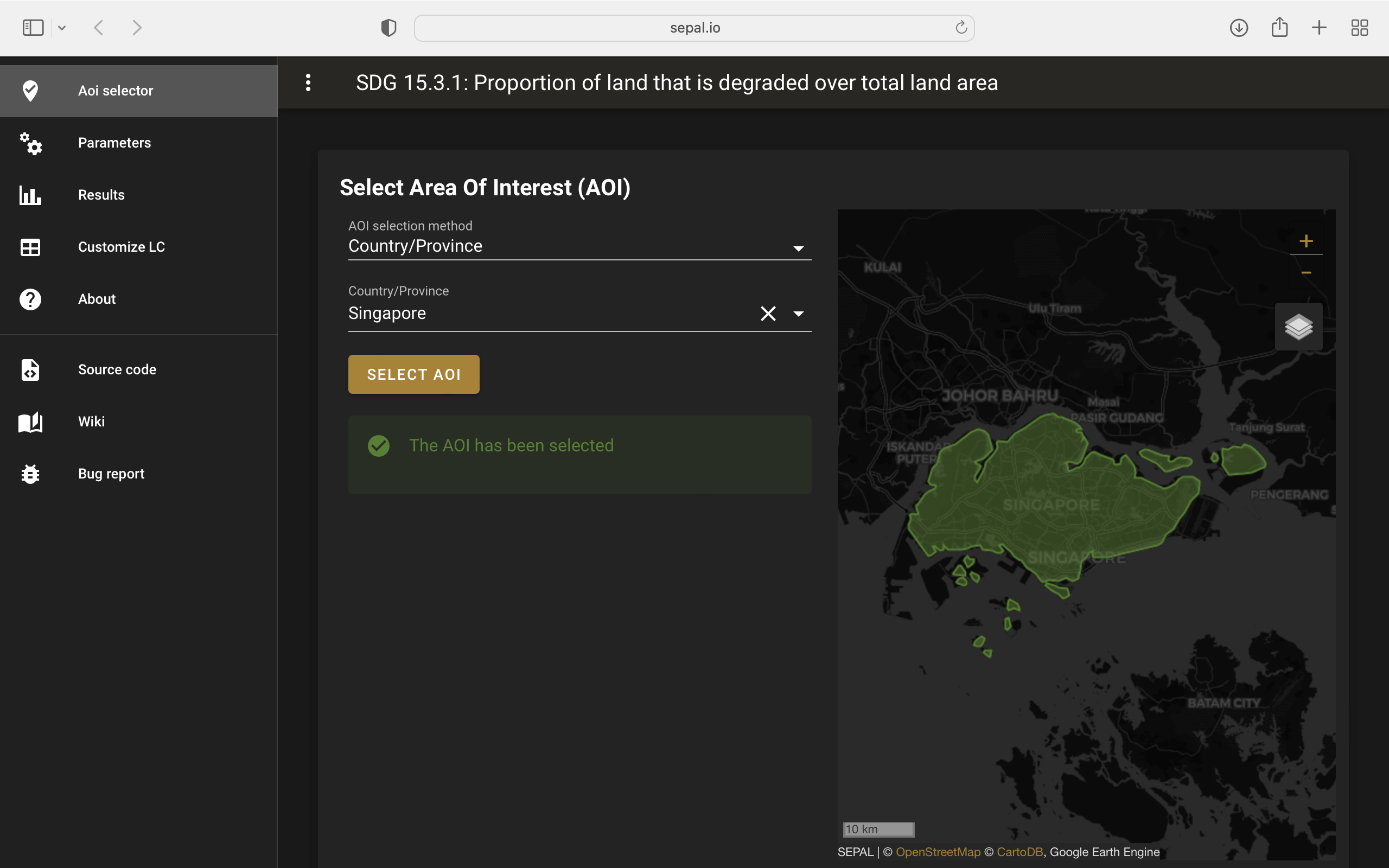
Select an AOI

SDG indicator 15.3.1 will be calculated based on user inputs. The first mandatory input is the area of interest (AOI).

In this step, you can choose from a predefined list of administrative layers or use your own datasets. The available options include:

Predefined layers

• Country/province

• Administrative level 1

• Administrative level 2

Custom layers

• Vector file

• Drawn shapes on the map

• Google Earth Engine (GEE) asset

After choosing the desired area, select Select these inputs for the map to show your selection.

Note

You can only select one AOI. In some cases, depending on input data, you could run out of resources in GEE.

Parameters

To run the computation of SDG Indicator 15.3.1, several parameters need to be set.

To better understand the parameters required to calculate the SDG 15.3.1 Indicator and its sub-indicators, see Good practice guidance: SDG Indicator 15.3.1 – Proportion of land that is degraded over total land area (Version 2.0).

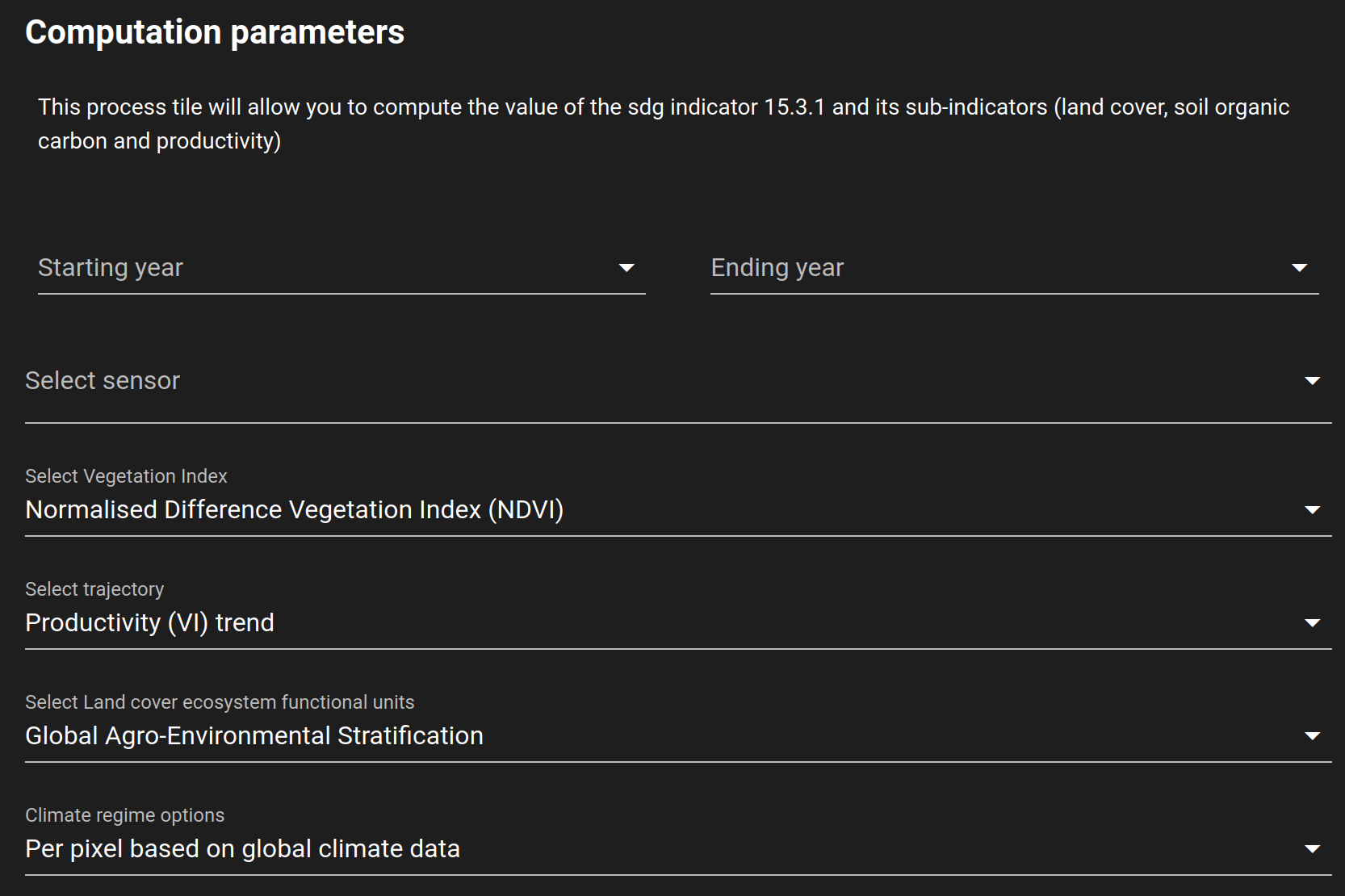
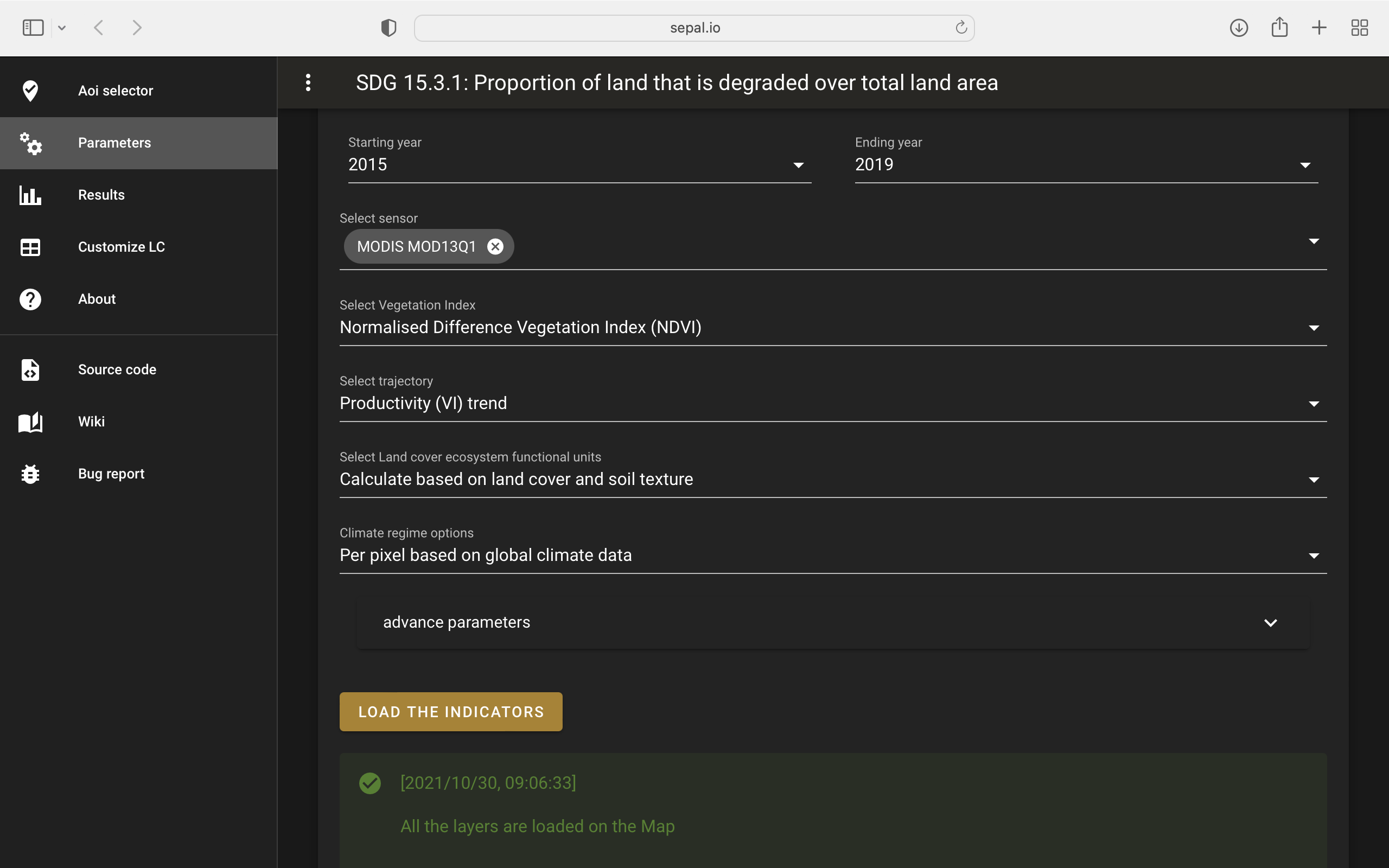
Mandatory parameters

• Assessment period: Set in years and must be in the correct order. The Starting year that you select will update the list of available sensors. You won’t be able to choose sensors that were not launched by the Ending year.

Note

In a strictly technical sense, the Productivity state metric assessment period should be longer than four years (historical plus the last three years). However, the assessment time frame for each of the sub-indicators and metrics is customizable in the Advanced parameters section.

• Sensors: After selecting the dates, all available sensors within the timeframe will be available. You can deselect or reselect any sensor you want. The default value is set to all Landsat satellites available within the selected timeframe.

Note

Some of the sensors are incompatible with others. Thus selecting Landsat, MODIS or Sentinel datasets in the Sensors dropdown menu will deselect the others.

• Vegetation index: The vegetation index will be used to compute the trend trajectory (by default: NDVI).

• Trajectory: There are three options available to calculate the productivity trend that describe the trajectory of change (by default, Productivity (VI) trend).

• Land ecosystem functional unit: Defaults to Global Agro-Environmental Stratification (GAES); other available options include:

  • Global Agro Ecological Zones (GAEZ), historical AEZ with 53 classes;

  • World Ecosystem;

  • Global Homogeneous Response Units; and

  • Calculate based on the land cover (ESA CCI) and soil texture (ISRIC).

• Climate regime: Defaults to Per pixel based on global climate data; however, you can also use a fixed value everywhere using a predefined climate regime in the dropdown menu or select a custom value with the slider.

Advanced parameters

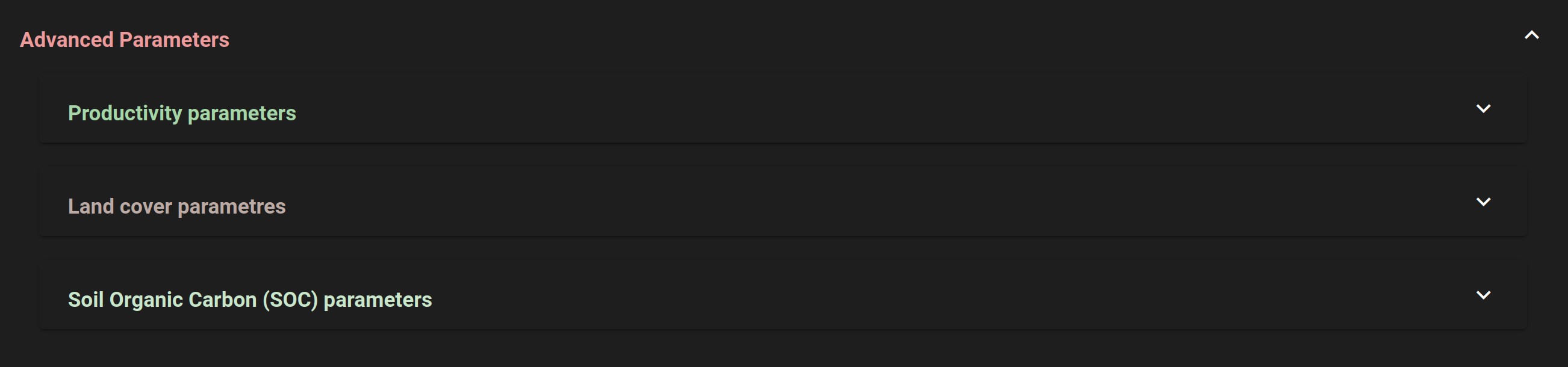
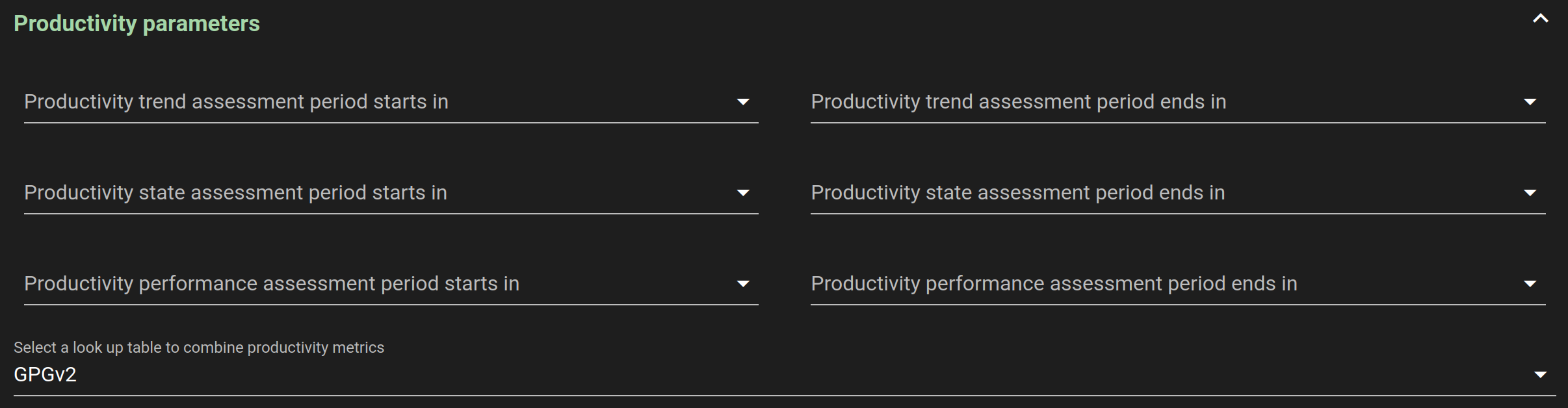
Productivity parameters

Assessment periods for all metrics can be specified individually. Keep them blank to use the start and end dates for the respective metric.

Note

If the start and end years you’ve chosen for your assessment period aren’t at least four years apart, you’ll need to choose an assessment period for the productivity state that’s longer. The module will disregard the value of a particular metric if you only specify the start or end year.

The default productivity “look-up” table is set to the second version of the good practice guidance, but you can also select the first version (to learn more about the “look-up” table, see the approach section for the tables and Section 4.2.5 of the the second version of the good practice guidance).

Land cover parameters

Water body data

The default water body data is set to JRC water body seasonality data with a seasonality of eight months. An ee.Image can be used for water body data with a pixel value greater than or equal to 1. A water body can be extracted from the land cover data by specifying the corresponding pixel value. Set the slider to 70 to use the water body extent from ESA CCI land cover data in case of default land cover and land cover data using UNCDD land cover categories (default matrix).

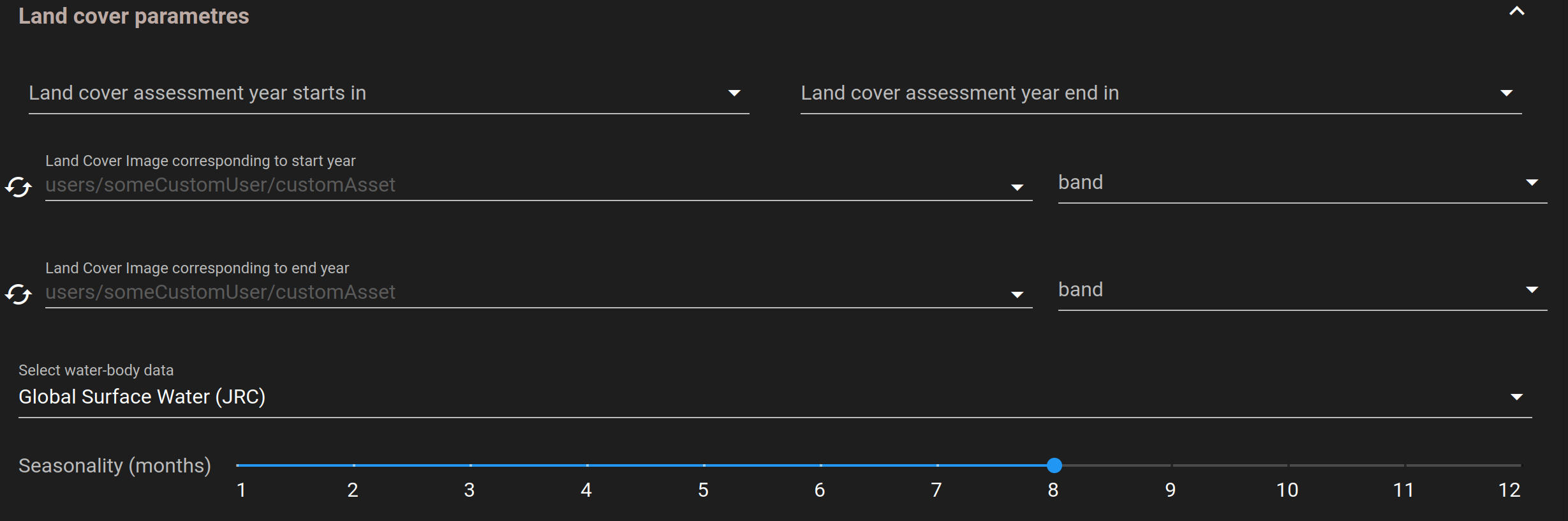
The default land cover is set to ESA CCI land cover data. The tool will use the CCI land cover system of the start date and end date. These land cover images will be reclassified into the UNCCD land cover categories and used to compute the land cover sub-indicator. However, you can specify your own data for the start and end land cover data. Provide the ee.Image asset name and the band that needs to be used, and the default dataset will be replaced in the computation with the specified land cover data.

Note

If you would like to use the default land cover transition matrix, the custom dataset needs to be classified in the UNCCD land cover categories. Please refer to Reclassify to know how to reclassify the local dataset into different classification systems.

To compute the land cover sub-indicator with the UNCCD land cover categories, the user can modify the default transition matrix. Based on the user’s local knowledge of the conditions in the study area and the land degradation process occurring there, use the table below to identify which transitions correspond to degradation (D), improvement (I), or no change in terms of land condition (S).

The rows stand for the initial classes and the columns for the final classes.

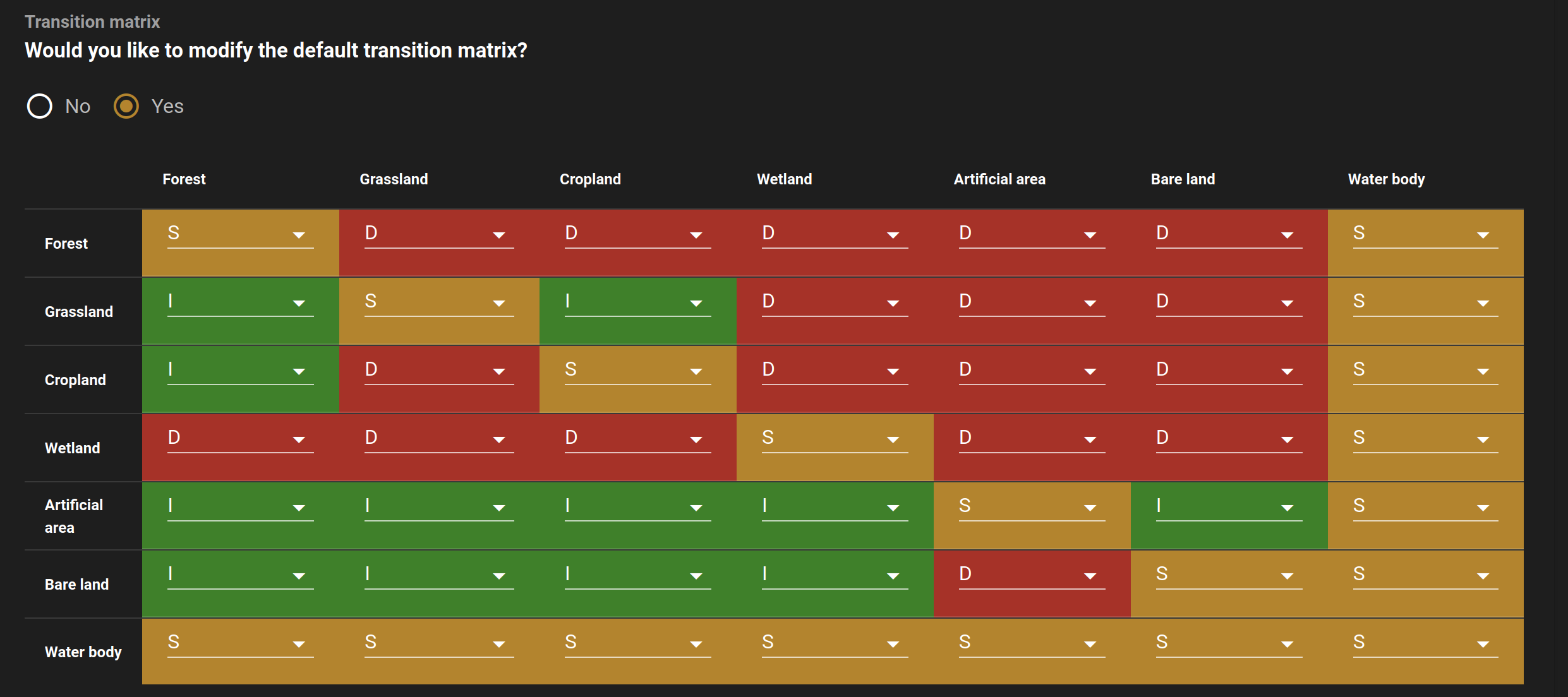
Custom land cover transition matrix

If you would like to use a custom land cover transition matrix, select the Yes radio button and the .csv file. Use this matrix as a template to prepare a matrix for your land cover map.

Tip

The module varifies land cover pixel values with values mentioned in the transition matrix. If there are missing class(es) in your land cover data, turn off Verify land cover pixel to bypasss the exact matching of pixel values.

SOC parameters

Launch the computation

Once all parameters are set, run the analysis by selecting Load the indicators.

It takes time to calculate all sub-indicators. Follow the progress in the lower panel.

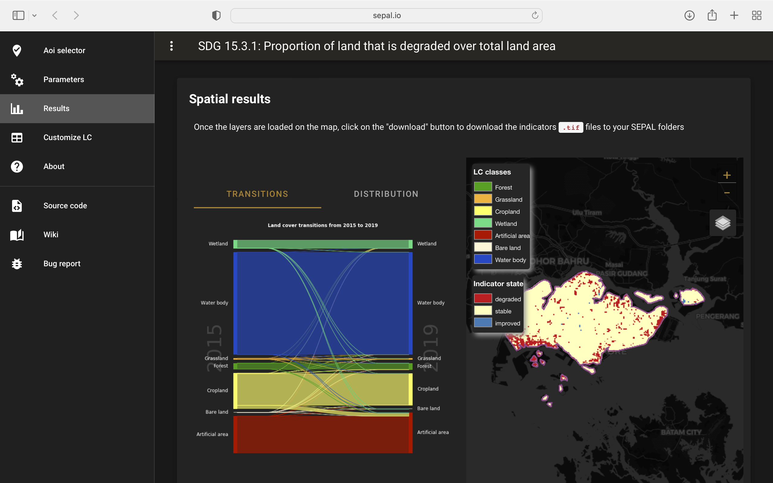
Results

The results are displayed to the end user in the next panel. On the left, the user will find the transition and distribution charts; on the right, an interactive map where every indicator and sub-indicators are displayed.

Select the download button to export all layers, charts and tables to your SEPAL folder.

The results are gathered in the module_results/sdg_indicators/ folder. Within this folder, a folder is set for each AOI (e.g. SGP/ for Singapore); within this folder results are grouped by run computation. The title of the folder reflects the parameters following this symbology: <start_year>_<end_year>_<satellites>_<vegetation index>_<lc units>_<custom LC>_<climate>.

Note

As an example for computation used in this documentation, the results were saved in: module_results/sdg_indicator/SGP/2015_2019_modis_ndvi_calculate_default_cr0/

Note

The results are interactive. Interact with charts and map layers using the widgets.

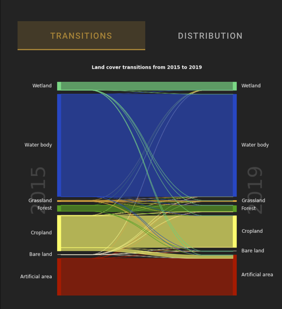
Transition graph

This chart is the Sankey diagram of the land cover transition between the baseline and target year. The colour corresponds to the initial class.

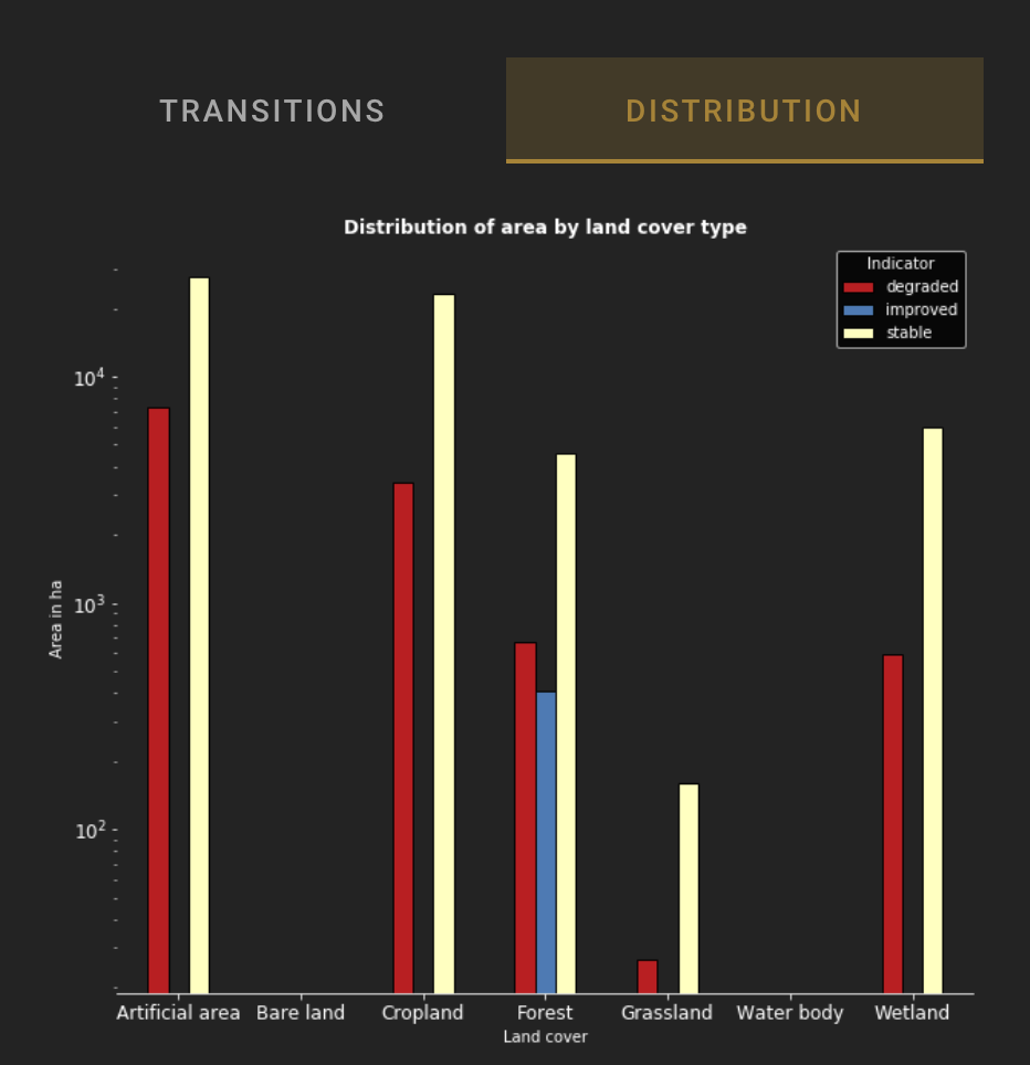
Distribution graph

This chart displays the distribution of SDG Indicator 15.3.1 by land cover classes.

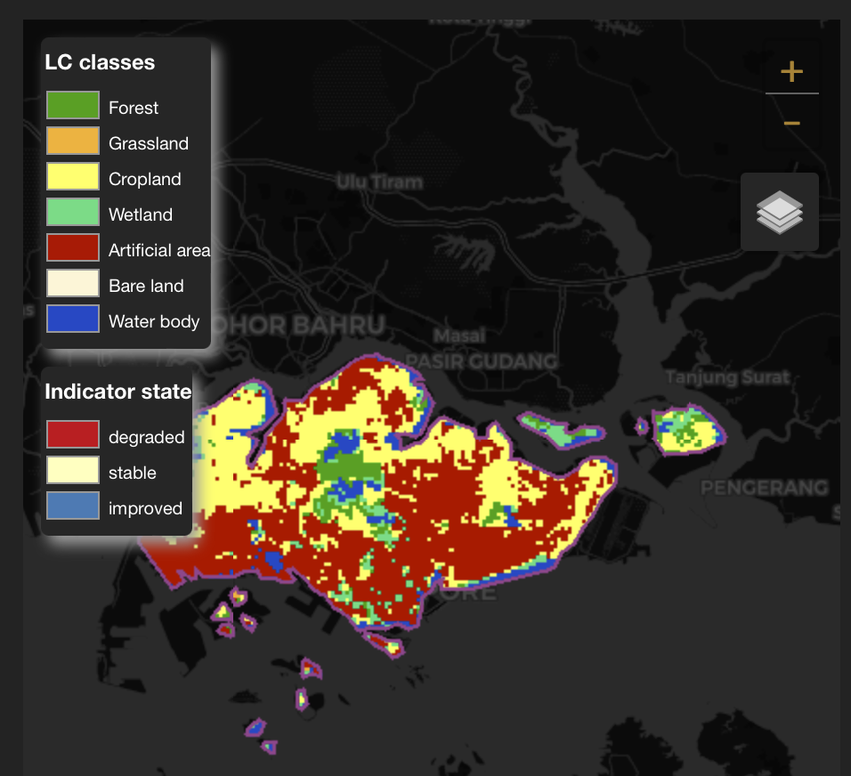
Interactive map

The following layers are available on the interactive map:

• Final indicator SDG 15.3.1

• Land cover sub-indicator

• Productivity sub-indicator

• Land cover sub-indicator

• SOC sub-indicator

• Land cover maps

• AOI

Reclassify

Attention

To reclassify land cover data, it needs to be available to the user as an ee.Image in GEE.

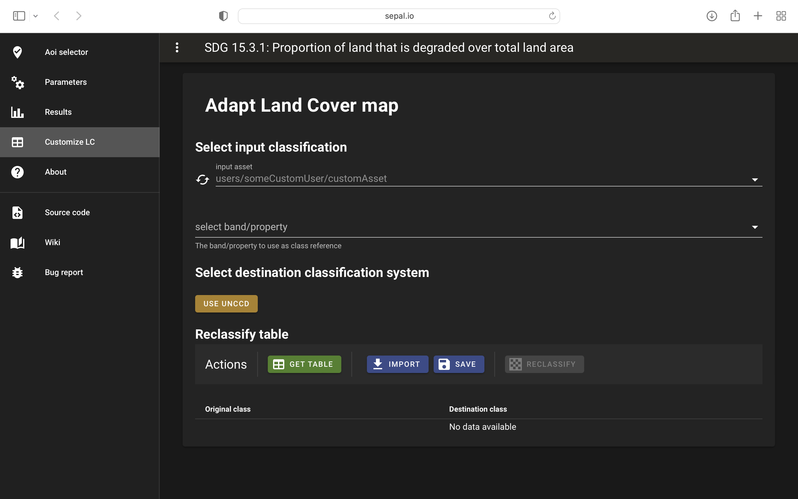
In order to use a custom land cover map, the user needs to first reclassify to a classification system.

First, select the asset in the combobox. It will be part of the dropdown value if the asset is part of the user’s asset list. If that’s not the case, set the name of the asset in the TextField.

Then, select the band that will be reclassified.

For the default UNCCD land cover categories, values between 10 to 70 are used to describe the following land cover classes:

1. Tree-covered areas (10)

2. Grassland (20)

3. Cropland (30)

4. Wetland (40)

5. Artificial surface (50)

6. Other lands (60)

7. Water bodies (70)

These categories are specified in the default UNCCD classification system. For a custom legend/classification system, upload a matrix with: the first column as pixel values; second column as class label; and third coloumn as colour code in HEX format. An example is given below:

21	Rural settlement	#005CE6
22	Mixed plantation	#FFFFBE
23	Urban settlement	#FFAA00
24	Mines	#F2D9BF
25	Bare soil	#E6E600
26	Rivers	#2699CC
27	Lake	#40B3FF
28	Mangrove	#5C8944
29	Forest	#B3FF80
30	Cropland	#704489
31	Grassland	#99FF00
32	Orchard	#1DBD9C

Note

This band needs to be a categorical band; the reclassification system won’t work with continuous values.

Select get table to generate a table with all categorical values of the asset. In the second column, set the destination value.

Tip

• If the destination class is not set, the class will be interpreted as “no_ata” (i.e. 0).

• Select save to save the reclassification matrix. It’s useful when the baseline and target map are in the same classification system.

• Select import to import a previously saved reclassification matrix.

Select reclassify to export the map in GEE using the IPCC classification system. The export can be monitored in GEE.

The following .gif will show you the full reclassification process with a simple example.