

Time series#
Create and retrieve SITS to study patterns and key changes in landscape evolution over time
Overview#
A Satellite Image Time Series (SITS) is a set of satellite images taken of the same scene at different times. A SITS makes use of different satellite sources to obtain a larger data series with a short time interval between two images. In this case, it is fundamental to observe the spatial resolution and registration constraints.
Satellite observations offer opportunities for understanding how the Earth is changing, determining the causes of these changes and predicting future changes. Remotely sensed data, combined with information from ecosystem models, offer an opportunity for predicting and understanding the behaviour of Earth’s ecosystems. Sensors with high spatial and temporal resolutions make the observation of precise spatio-temporal structures in dynamic scenes more accessible. Temporal components integrated with spectral and spatial dimensions allow the identification of complex patterns concerning applications connected with environmental monitoring and analysis of land cover dynamics.
Change detection can only provide a “before and after” scenario; a time-series analysis provides an opportunity to study patterns and key changes in the landscape evolution over time.
This SEPAL recipe allows users to create and retrieve SITS based on Landsat and Copernicus programmes’ imagery using the Google Earth Engine (GEE) datacube.
Attention
You won’t be able to download images if your SEPAL and GEE account aren’t connected. To learn more, go to Connect SEPAL to GEE.
Start#
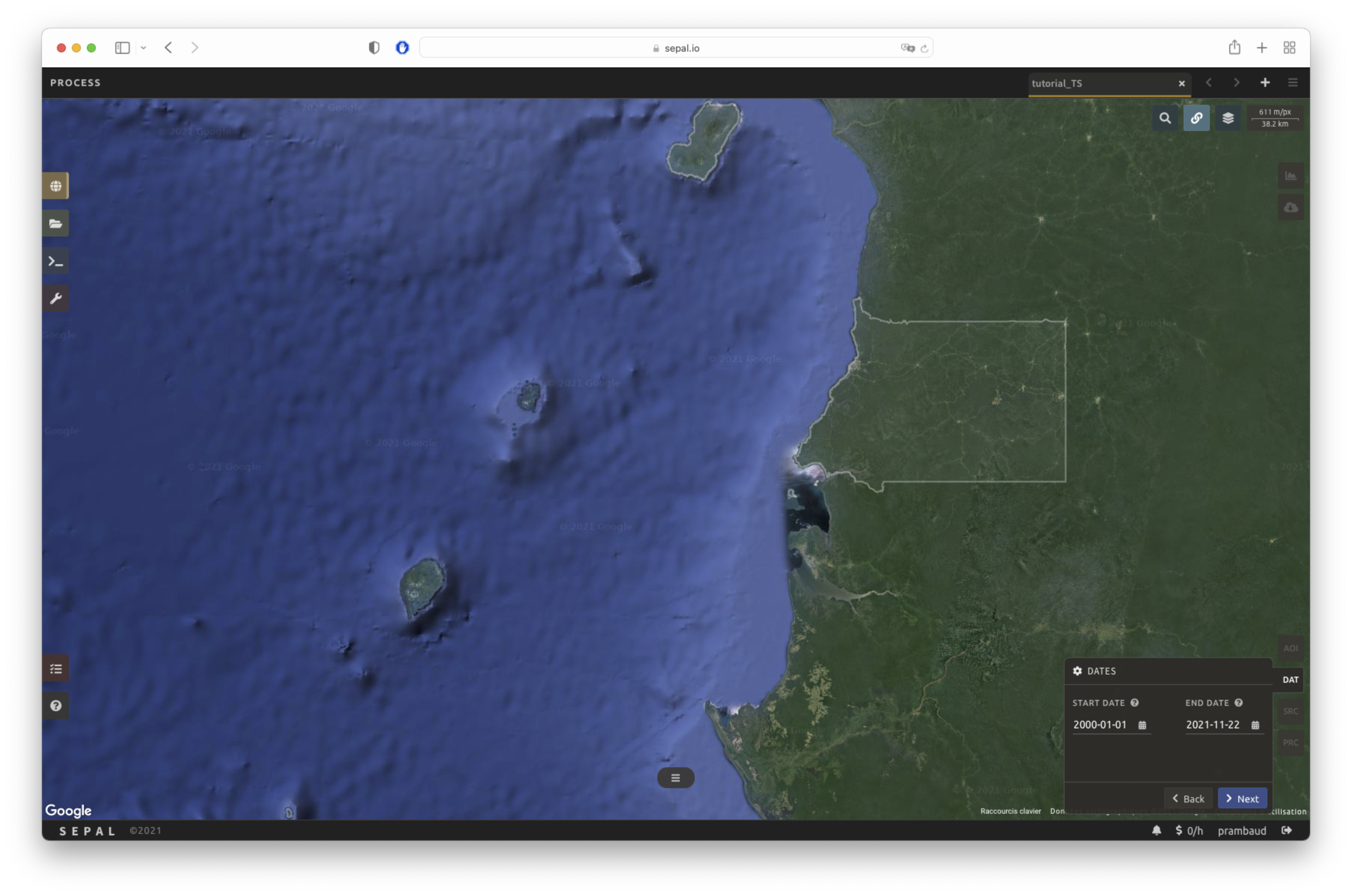
Once the Time series recipe is selected, SEPAL will open the recipe process in a new tab (see 1 in the following figure). The base map will change to Google high-resolution imagery and the Area of interest (AOI) selection window will appear in the lower right (2).
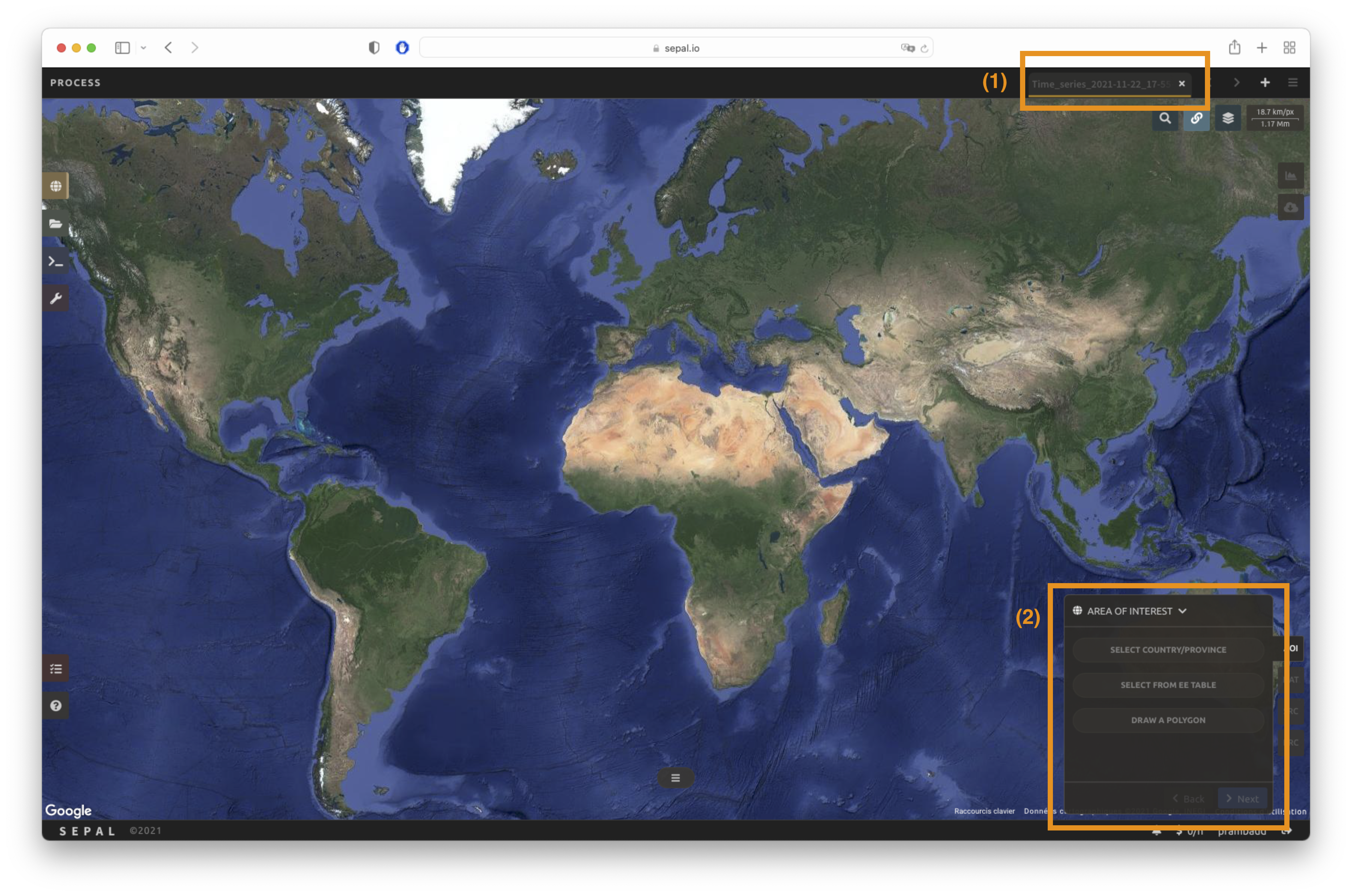
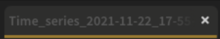
The first step is to change the name of the recipe. This name will be used to identify your files and recipes in the SEPAL folders. Use the best-suited convention for your needs. Simply double-click the tab and enter a new name. It will default to Time_series_<start_date>_<end_date>_<band name>.

Note
The SEPAL team recommends using the following naming convention: <aoi name>_<start-<end>_<measure>_<sensors> (e.g. sgp_2012-2018_ndfi_l78).
Parameters#
In the lower-right corner, four tabs are available, allowing you to customize the time series to your needs:
AOI: area of interest (AOI)
DAT: dates of the time series
SRC: source datasets of the time series
PRC: pre-processing parameters
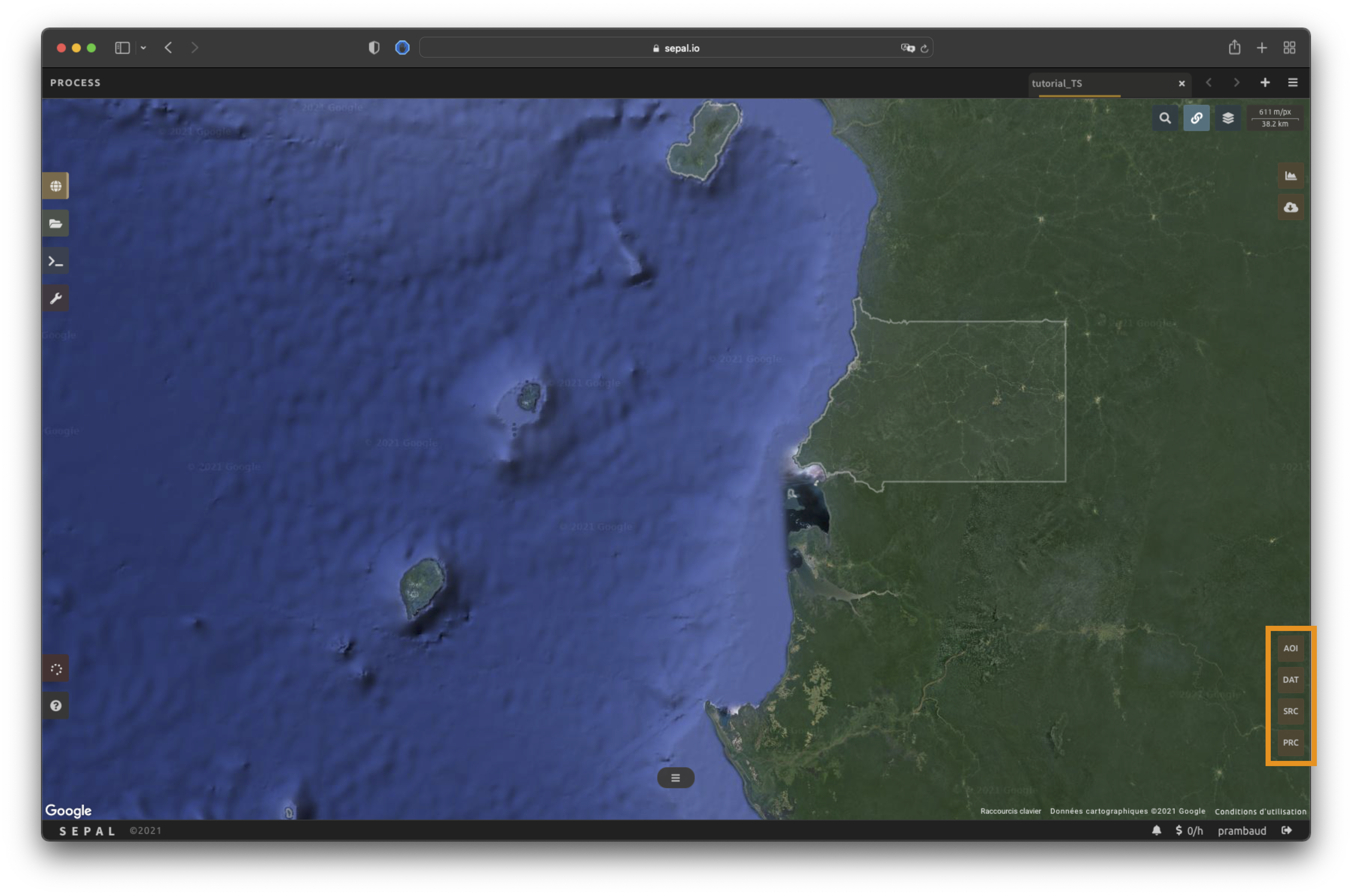
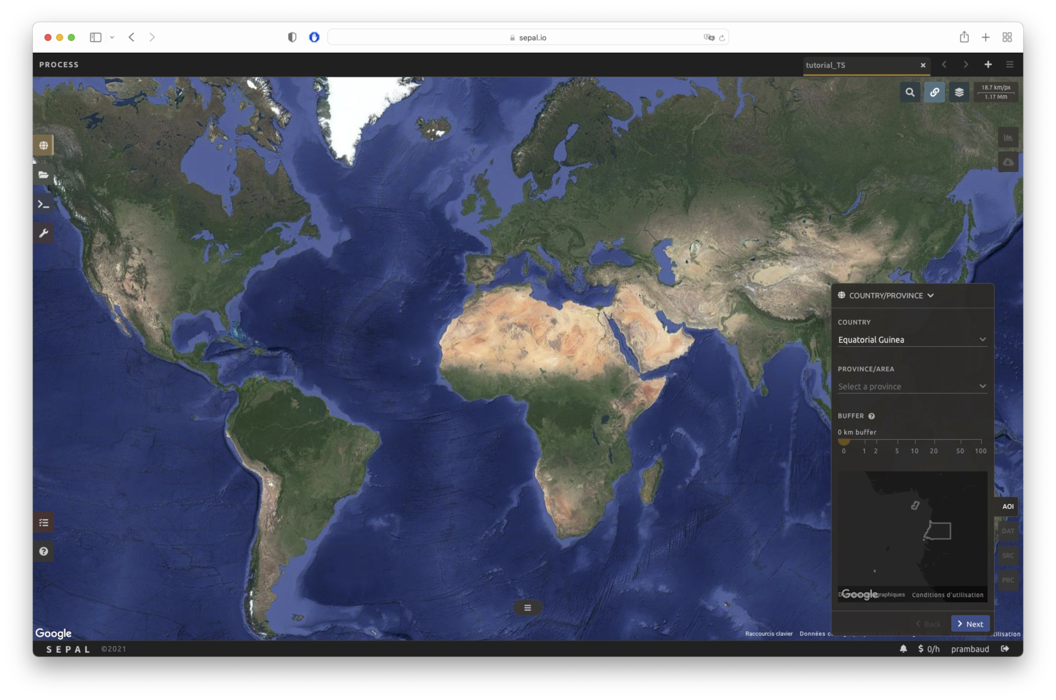
AOI selection#
The data exported by the recipe will be confined to the bounds of the AOI. There are multiple ways to select the AOI in SEPAL:
Administrative boundaries
EE Tables
Drawn polygons
For more information, go to AOI selection.
Dates#
In the DAT tab, you will be asked to select the start date and end date of the time series. Select the Date text field to open a pop-up window. Choose the Select button to choose a date. When both dates have been chosen, select the Apply button.

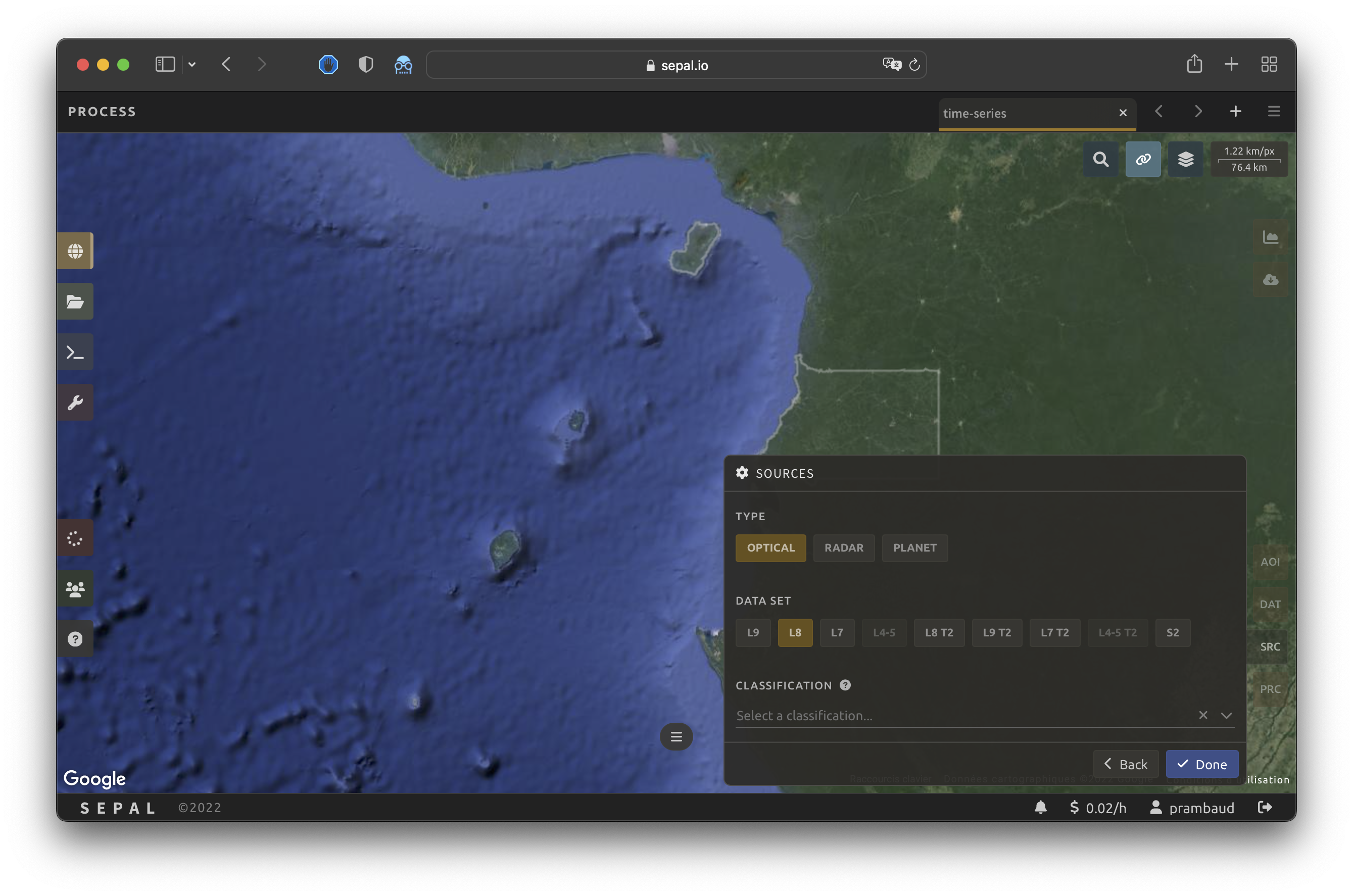
Sources#
As mentioned in the introduction, a SITS makes use of different satellite sources to obtain a larger data series with a shorter time interval between the images. To meet this objective, SEPAL allows you to select data from multiple entry points. You can select multiple sources from Radar, Optical or Planet datasets.
When all of the data has been selected, select Apply.
Pre-processing#
Note
This section is optional as these parameters are set by default.
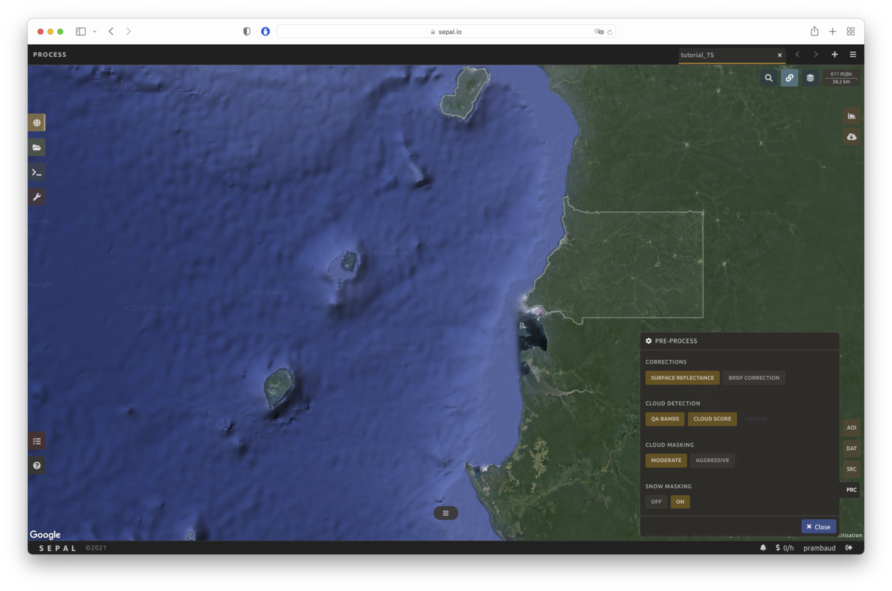
Correction:
NoneCloud detection: QA bands, Cloud score
Cloud masking: moderate
Snow masking: on
Multiple pre-processing parameters can be set to improve the quality of the provided images. SEPAL has gathered four of them in the form of these interactive buttons. If you think others should be added, tell us in the issue tracker.
Correction
Surface reflectance: Use scenes’ atmospherically corrected surface reflectance.
BRDF correction: Correct for bidirectional reflectance distribution function (BRDF) effects.
Cloud detection
QA bands: Use previously created quality assessment (QA) bands from datasets.
Cloud score: Use a cloud-scoring algorithm.
Cloud masking
Moderate: Rely only on image source QA bands for cloud masking.
Aggressive: Rely on image source QA bands and a cloud-scoring algorithm for cloud masking (this will probably “mask” some built-up areas and other bright features).
Snow masking
On: Mask snow (this tends to leave some pixels with shadowy snow).
Off: Don’t mask snow (some clouds might get misclassified as snow, and because of this, disabling snow masking might lead to cloud artefacts).
Available bands#
Note
The wavelength of each band is dependent on the satellite used.
The time series will use a single observation for each pixel. This observation can be one of the available bands in SEPAL. To discover the full list of available bands, see Optical Satellite bands, transformations, and indices and ../feature/radar_bands.
Analysis#
Once all parameters are set, you can generate data from the recipe. Some can be directly generated on the fly from the interface; the rest require retrieving the data from SEPAL folders.
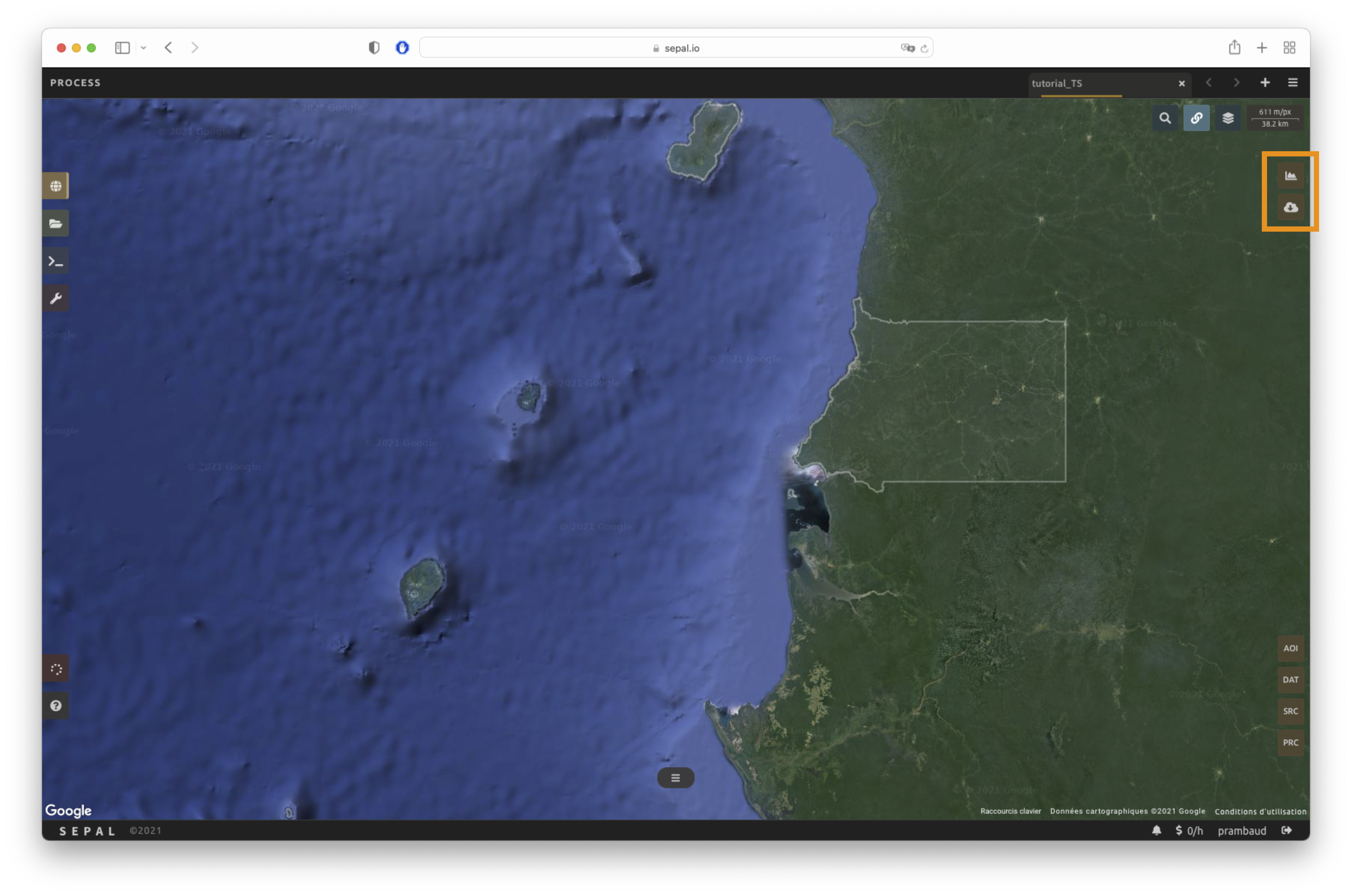
The analysis icons can be found in the upper-right corner of the SEPAL interface:
: Plot data.
: Retrieve data.
Tip
The Download icon is only enabled when the data parameters are complete. If the button is disabled, check your parameters, as some might be missing.
Plot#
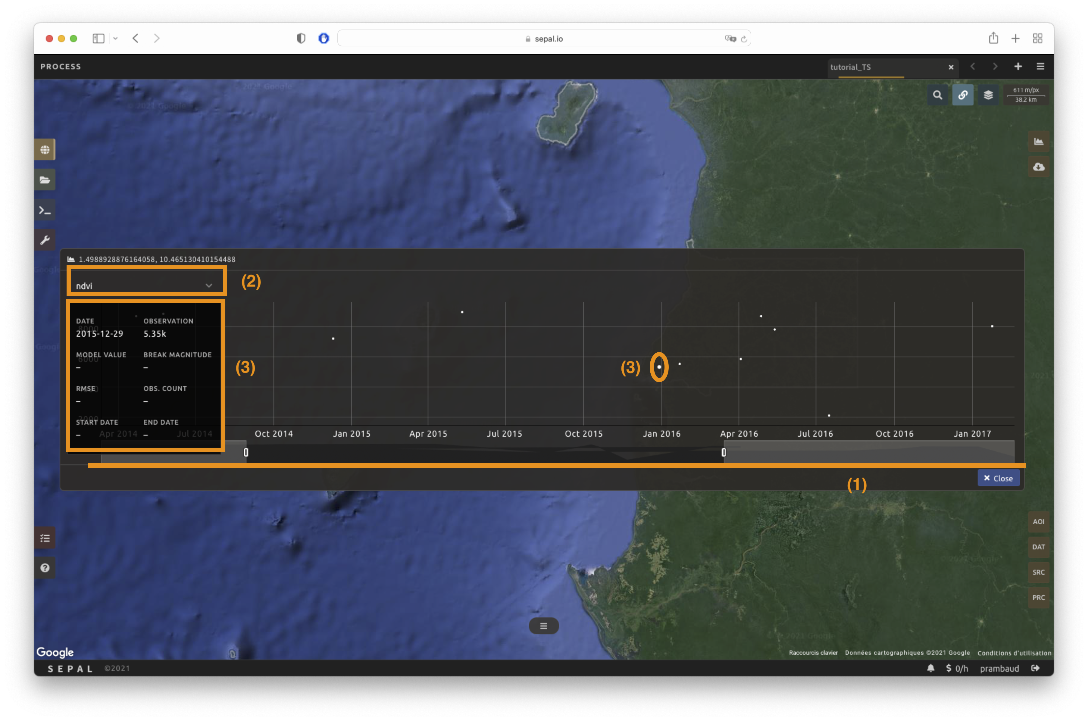
Select to start the plotting tool. Move the pointer to the main map; the pointer will be transformed into a . Click anywhere in the AOI to plot data for this specific location in the following pop-up window.
The plotting area is dynamic and can be customized by the user.
Using the slider (1), the temporal width displayed can be changed. It cannot exceed the start and/or end date of the time series.
You can also select the observation feature by selecting one of the available measures in the dropdown selector in the upper-left corner (2). The available bands are the same as those described previously.
On the main graph, each point represents one valid observation (based on the pre-processing filters). Hover over the point to let the tooltip describe the value and date of the observation (3).
Tip
The coordinates of the point are displayed at the top of the chart window.
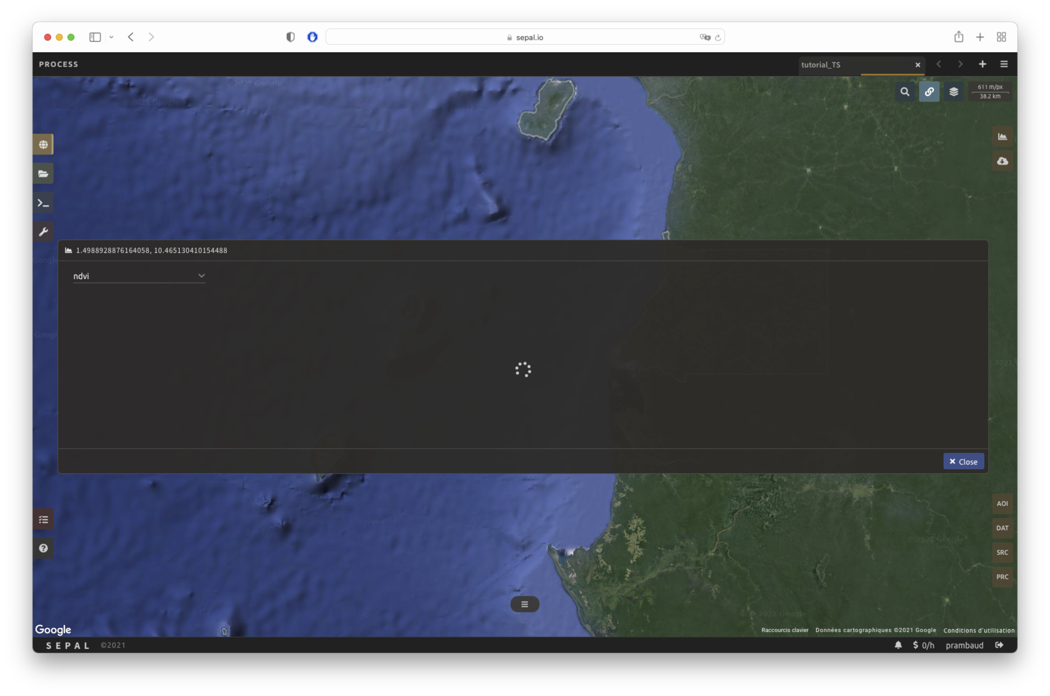
Attention
Since the plot feature is retrieving information from GEE on the fly and presenting it in an interactive window, this operation can take time, depending on the number of available observations and the complexity of the selected pre-processing parameters. If a spinning wheel appears in the pop-up window, you may have to wait up to two minutes to see the data displayed.
Export#
In order for the data generated by the recipe to be used in other workflows, it needs to be retrieved from GEE and uploaded to SEPAL.
Important
You cannot export a recipe as an asset or a .tiff file without a small computation quota. If you are a new user, see Manage your resources.
Parameters#
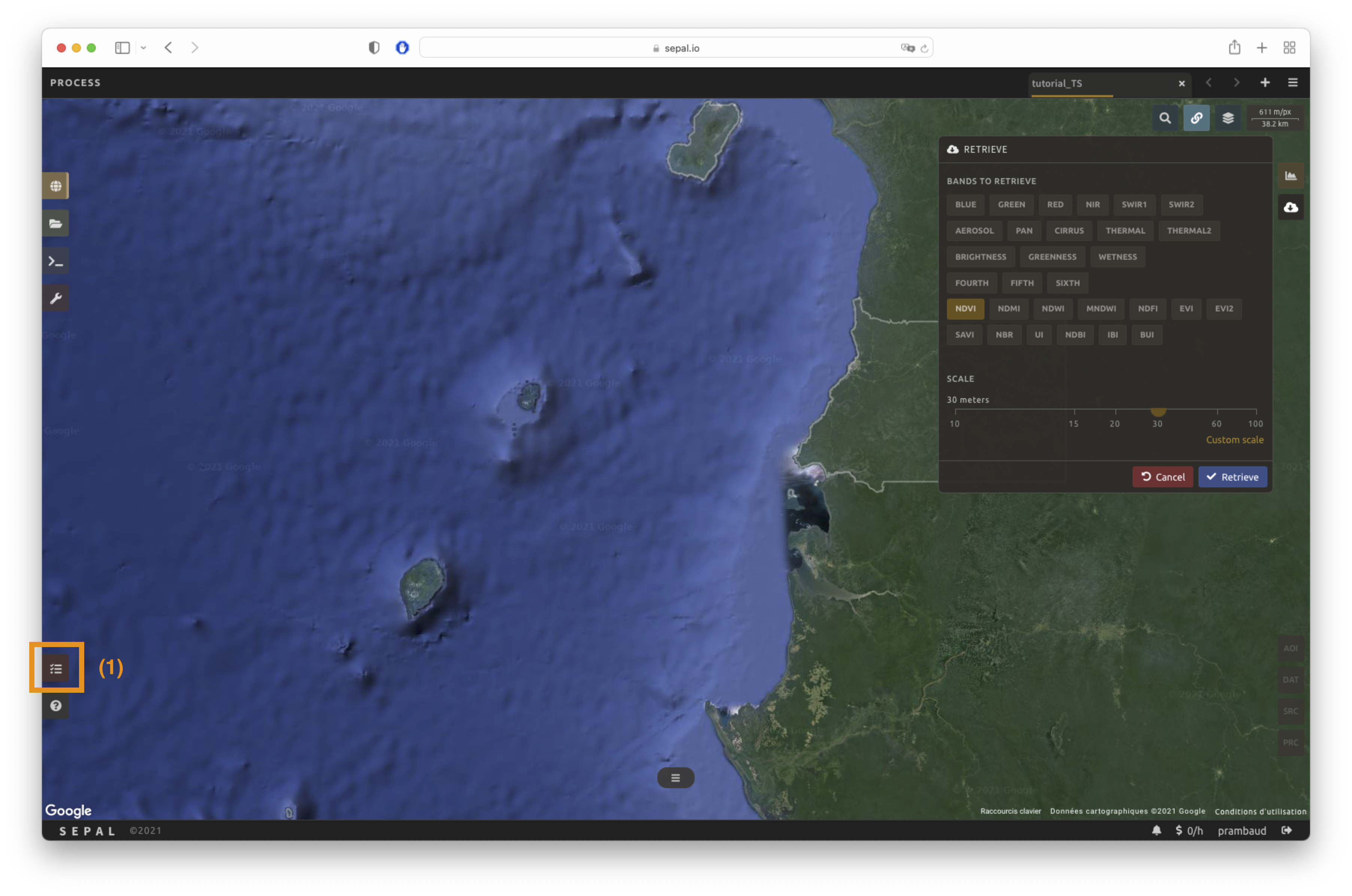
Select to open the Download parameters window. You will be able to select the measure to use on each observation of the time series. This measure can be selected in the list of available bands presented above in a previous section.
Note
There is no fixed rule to the measure selection. Each index is more adapted to a set of analyses in a defined biome. The knowledge of the study area, the evolution expected and the careful selection of an adapted measure will improve the quality of downstream analysis.
You can set a custom scale for exportation by changing the value of the slider in metres (m). Keep in mind that Sentinel data native resolution is 10 m and Landsat is 30 m.
When all the data is selected, select the apply button. Notice that the task tab in the lower-left corner of the screen (1) will change from to , meaning that the tasks are loading.
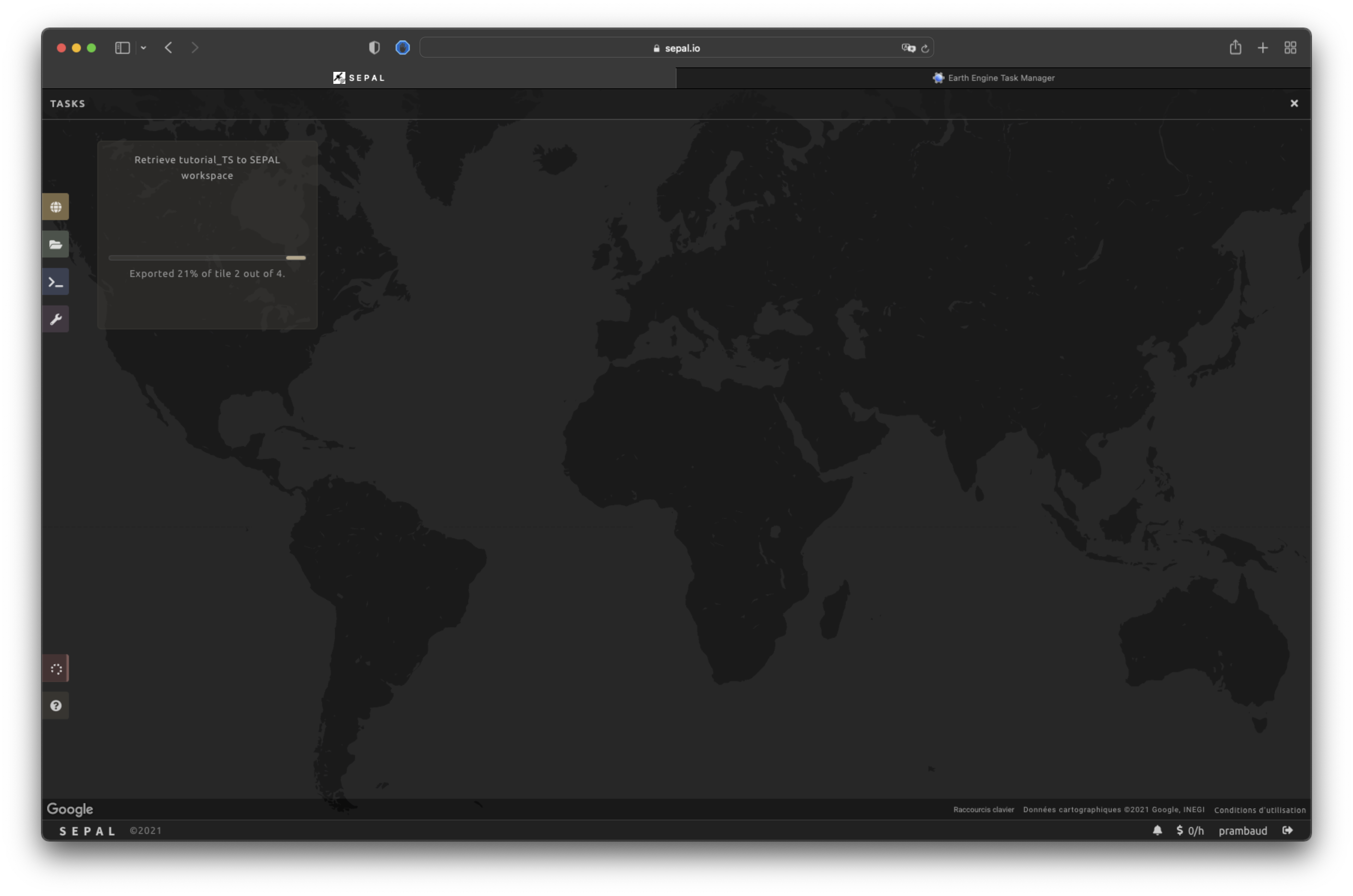
Exportation status#
By selecting the Tasks tab (lower-left corner using the or buttons, depending on the loading status), you will see the list of different tasks loading. The interface will provide you with information about the task progress and display an error if the exportation has failed. If you are unsatisfied with the way we present information, the task can also be monitored using the GEE task manager.
Tip
This operation is running between GEE and SEPAL servers in the background, so you can close the SEPAL page without ending the process.
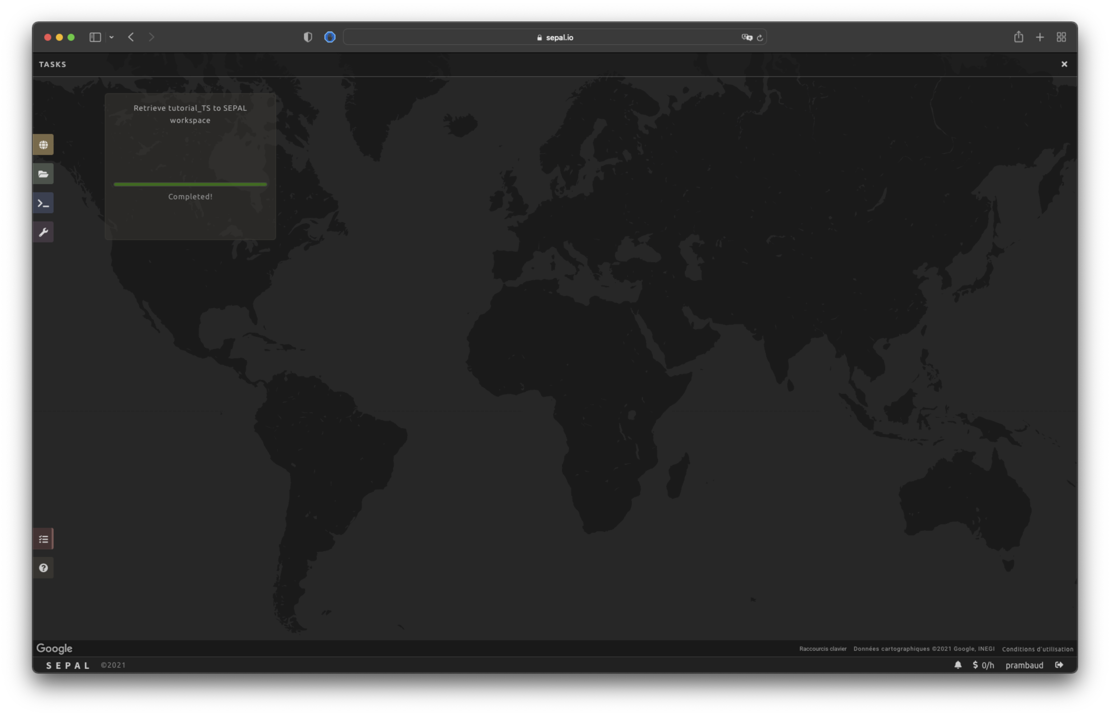
When the task is finished, the frame will be displayed in green, as shown in the second image below.
Access#
Once the download process is done, you can access the data in your SEPAL folders in Downloads, using the following format:
.
└── downloads
    └── <TS name>
        ├── <tile number>
        │   ├── chunk-<start date>_<end date>
        │   │   ├── <TS name>_<tile number>_<start_date>_<end date>-<gee tiling id>.tif
        │   │   ├── ...
        │   │   └── <TS name>_<tile number>_<start_date>_<end date>-<gee tiling id>.tif
        │   ├── ...
        │   ├── chunk-<start date>_<end date>
        │   ├── tile-<gee tiling id>
        │   │   └── stack.vrt
        │   ├── ...
        │   ├── tile-<gee tiling id>
        │   ├── dates.csv
        │   └── stack.vrt
        ├── ...
        └── <tile number>
Important
Understanding how images are stored in a time series is only required if you want to manually use them. The SEPAL applications are bound to this tiling system and can digest this information for you.
The data are stored in a folder using the name of the time series as it was labeled in the first section of this document. The SEPAL team was forced to use this folder structure as GEE is unable to export an ee.ImageCollection. As the data is spatially too big to be exported at once, they are divided into smaller pieces and reassembled in a stack.vrt file.
The AOI provided by the user will be divided into multiple SEPAL tiles. The AOI is a ee.FeatureCollection; each feature is downloaded in a different tile. If the tile is bigger than 2° x 2° (EPSG:4326), then the feature is divided again until all of the tiles are smaller than the maximum 2° size. The tiles are identified by their <tile_number>.
To limit the size of the downloaded images, in each SEPAL tile, the time period is divided into Chunks of 3 months. They are identified by their <chunk-<start>_<end>. Chunks are image folders. As a SEPAL tile is still bigger than what GEE can download at once, the images are divided into GEE tiles. This tiling process uses its own identification system (000000xxxx-000000xxxx). Consequently, Chunks contain tile raster images. Each one of these images is composed of one band per observation date, with the value of the measure for each pixel. The bands are named with the date.
To gather all these rasters together, a first aggregation on time is performed. One stack.vrt is created per GEE tile, meaning that each stack.vrt file contains all the *<gee tiling id>.tif contained in each Chunk, reconstituting the full time period on the smallest spatial unit: the GEE tile. Each file is stored in a folder called tile-<gee tiling id>.
Finally, information is gathered spatially at the SEPAL tile level in the main stack.vrt file.
The last file, date.csv, gathers all the observation dates in chronological order.
Note
The dates contained in date.csv can differ from one SEPAL tile to another, due to data availability and pre-processing filters.
Tip
The full folder with a consistent treefolder is required to read the .vrt
Here is an example of a real TS folder:
.
└── downloads
    └── tutorial_TS
        ├── 1
        │   ├── chunk-2012-01-01_2012-04-01
        │   │   ├── tutorial_TS_1_2012-01-01_2012-04-01-0000000000-0000000000.tif
        │   │   ├── ...
        │   │   └── tutorial_TS_1_2012-01-01_2012-04-01-0000002560-0000001024.tif
        │   ├── ...
        │   ├── chunk-2018-10-01_2018-12-31
        │   ├── tile-0000000000-0000000000
        │   │   └── stack.vrt
        │   ├── ...
        │   ├── tile-0000002560-0000001024
        │   ├── dates.csv
        │   └── stack.vrt
        ├── ...
        └── 3
Important
Now that you have downloaded the TS to your SEPAL account, it can be downloaded to your computer using FileZilla or used in one of our Time-series analysis modules.