

Classification#
Build supervised classifications of mosaic images to create easy-to-use user interfaces with the Classification recipe
Overview#
With this recipe, SEPAL helps users build supervised classifications of any mosaic image. It is built on top of the most advanced tools available on Google Earth Engine (GEE) – including seven classifiers, such as Random Forest, CART and SVM – allowing users to create an easy-to-use user interface to:
select an image to classify;
define the legend; and
add training data from external sources and on-the-fly selection.
In combination with other tools of SEPAL, the Classification recipe can help you provide accurate land-use maps, without writing a single line of code.
Start#
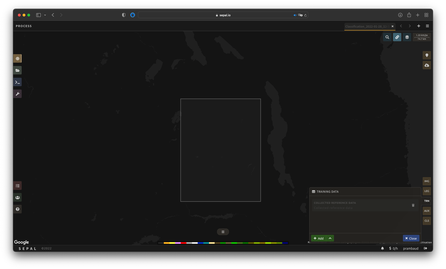
Once the Classification recipe is selected, SEPAL will show the recipe process in a new tab (see 1 in figure below); the Image selection window will appear in the lower right (2).
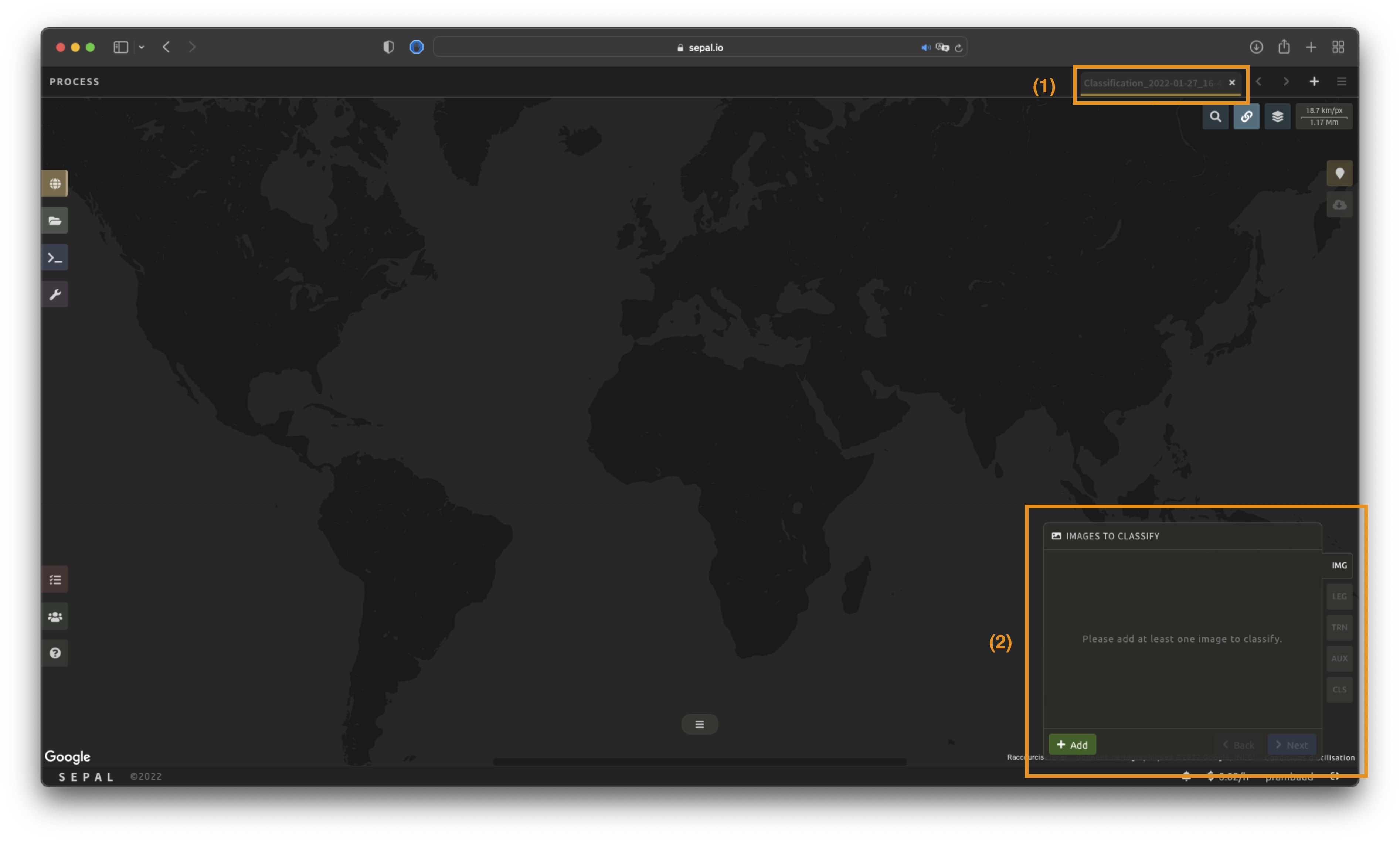
The first step is to change the name of the recipe. This name will be used to identify your files and recipes in SEPAL folders. Use the best-suited convention for your needs. Simply double-click the tab and enter a new name. It will default to Classification_<timestamp>.

Note
The SEPAL team recommends using the following naming convention: <image_name>_<classification>_<measures>.
Parameters#
In the lower-right corner, the following five tabs are available, allowing you to customize the classification to your needs:
IMG: image to classify
LEG: legend of the classification system
TRN: training data of the model
AUX: auxiliary global dataset to use in the model
CLS: classifier configuration

Image selection#
The first step consists of selecting the image bands on which to apply the classifier. The number of selected bands (i.e. images) is not limited.
Note
Keep in mind that increasing the number of bands to analyse will improve the model but slow down the rendering of the final image.
Note
If multiple images are selected, all selected images should overlap. If masked pixels are found in one of the bands, the classifier will mask them.
Select Add. The following screen should be displayed:
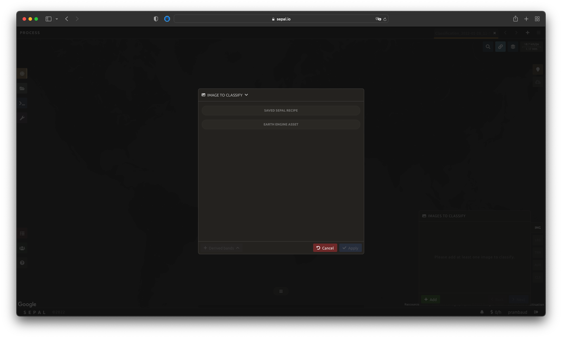
Image type#
Users can select images coming from a Saved SEPAL recipe or an exported Earth Engine asset (see advantages and disadvantages below). Both should be an ee.Image, rather than a Time series or ee.ImageCollection.
Saved SEPAL recipe:
Advantages:
all of the computed bands from SEPAL can be used; and
any modification to the existing recipe will be propagated in the final classification.
Disadvantages:
the initial recipe will be computed at each rendering step, slowing down the classification process and potentially breaking on-the-fly rendering due to GEE timeout errors.
Earth Engine asset:
Advantages:
can be shared with other users; and
the computation will be faster, as the image has already been exported.
Disadvantages:
only the exported bands will be available; and
the
Imageneeds to be re-exported to propagate changes.
Both methods behave the same way in the interface.
Select bands#
Tip
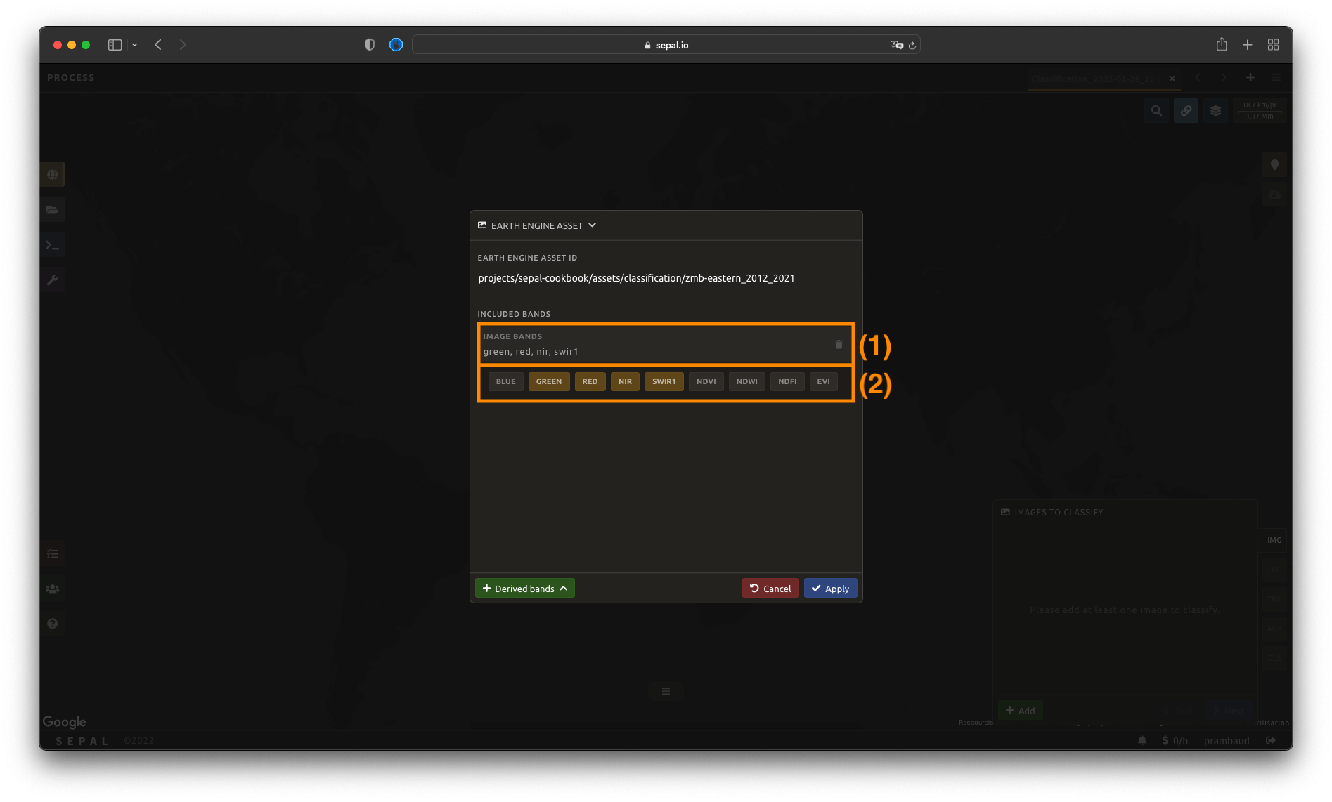
For this example, we will use a public asset created with the Optical mosaic tool from SEPAL. It’s a Sentinel-2 mosaic of Eastern Province in Zambia during the dry season from 2012 to 2021. Multiple bands are available.
Use the following asset name if you want to reproduce our workflow: projects/sepal-cookbook/assets/classification/zmb-eastern_2012_2021
Image bands#
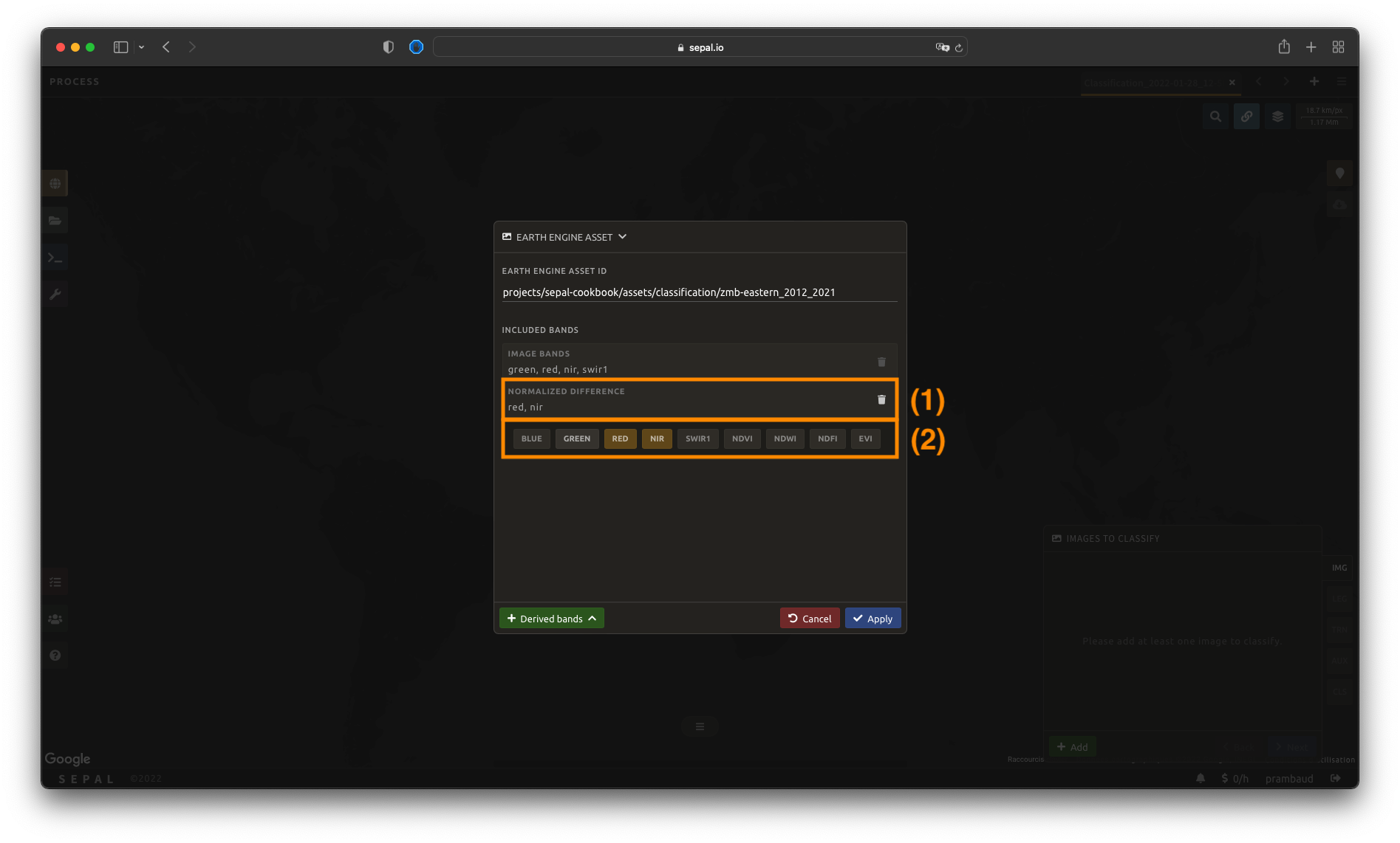
Once an asset has been selected, SEPAL will load its bands in the interface. You can use any band that is native to the image as input for the classification. Open the Select bands… dropdown and click a band name to add it (the highlighted option). Each selected band then appears as a removable chip in the Image bands panel.
In this example, we selected the following:
rednirswir1green
Derived bands#
The analysis is not limited to natively available bands. SEPAL can also build additional derived bands on-the-fly.
Select Derived bands at the bottom of the pop-up window and select the deriving method. This adds a new panel named after the selected method (e.g. Normalized difference). The method will be applied to the bands you add to that panel.
Note
If you select two bands, \(A\) and \(B\), and apply the Normalized difference derived band, you’ll add one band to your analysis:
\((A - B) / (A + B)\)
Selecting more than two bands applies the operation to each pair of them.
Note
You should notice that in the figure, we compute the normalized difference between nir and red (i.e. the NDVI). It is also pre-computed in the Indexes derived bands.
Once image selection is complete, select Apply and the pop-up window will close. The images and bands will be displayed in the IMG panel in the lower-right corner of the screen. By selecting the button, you will remove the image and its bands from the analysis altogether.
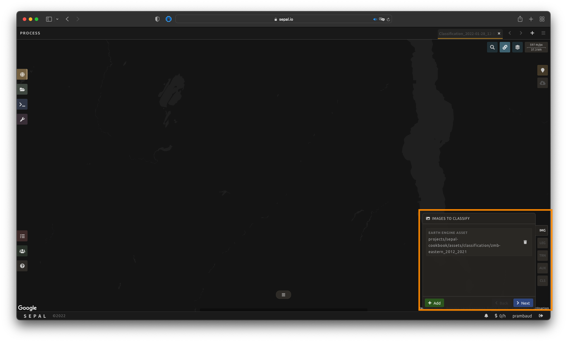
From there, select Next to continue to the next step.
Legend setup#
In this step, the user will specify the legend that should be used in the output classified image. Any categorical classification that associates integer value to a class name will work. SEPAL provides multiple ways to create and customize a legend.

Important
Legends created here are fully compatible with other functionalities of SEPAL, including applications.
Manual legend#
The first and most natural way of building a legend is to do it from scratch.
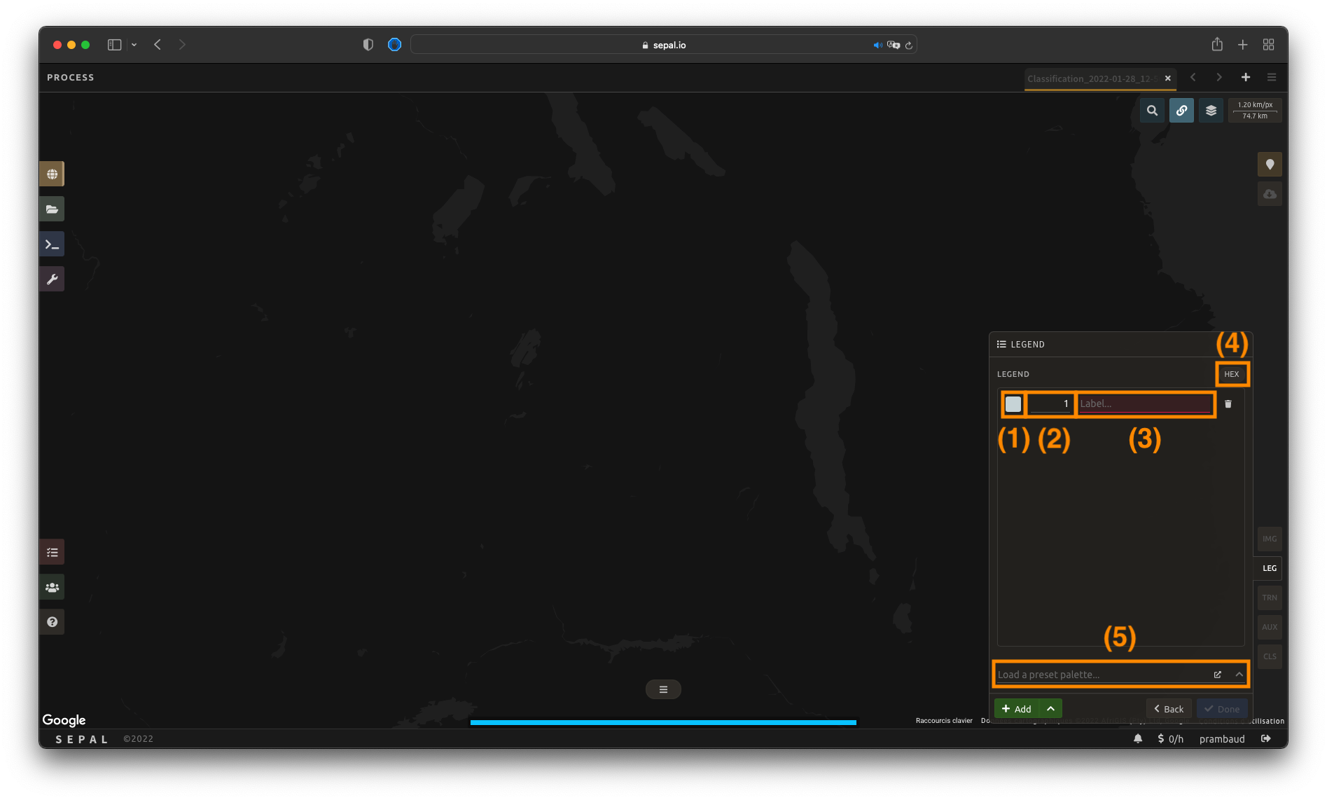
Select Add to add a new class to your legend.
A class is defined by three key elements:
Color (1): Select the small color square to open the color selector and choose any color (color[s] must be unique).
Value (2): Select any integer value (value must be unique).
Class (3): Insert a class description (cannot be empty).
Select the Add button again to add an extra class line. The button can be used to remove a specific line.
Tip
Select HEX (4) to display the hexadecimal value of the selected color. It can also be used to insert a known color palette by utilizing its values.
If multiple classes are created and you are not sure which one to use, you can apply colors to them by selecting a preselected color-map (5). They are provided by the GEE community and will be applied to every existing class in your panel.
Import legend#
If you already have a file describing your legend, you can use it, rather than identifying every legend item individually. Your legend needs to be saved in .csv format and contain the following information:
color (stored as a hexadecimal value [e.g. #FFFF00] or in three columns [red, blue, green]);
value (stored as an integer); and
class (stored as a string).
Note
The column names will help SEPAL predict information, but are not compulsory.
For example, a .csv file containing the following information is fully qualified to be used in SEPAL:
code,class,color
10,Tree cover,#006400
20,Shrubland,#ffbb22
30,Grassland,#ffff4c
40,Cropland,#f096ff
50,Built-up,#fa0000
60,Bare,#b4b4b4
70,Snow,#f0f0f0
80,Water,#0064c8
90,Herbaceous wetland,#0096a0
95,Mangroves,#00cf75
100,Moss,#fae6a0
Alternatively, a file containing the following information – including RGB-defined colors – is also acceptable:
code,class,red,blue,green
10,Tree cover,0,100,0
20,Shrubland,255,187,34
30,Grassland,255,255,76
40,Cropland,240,150,255
50,Built-up,250,0,0
60,Bare,180,180,180
70,Snow,240,240,240
80,Water,0,100,200
90,Herbaceous wetland,0,150,160
95,Mangroves,0,207,117
100,Moss,250,230,160
Once the fully qualified legend file has been prepared on your computer, select and then Import from CSV..., which will open a pop-up window where you can drag and drop the file or select it manually from your computer files.
As shown in the following image, you can then select the columns that are defining your .csv file (select Single column for hexadecimal-defined colors and Multiple columns for RGB-defined colors).
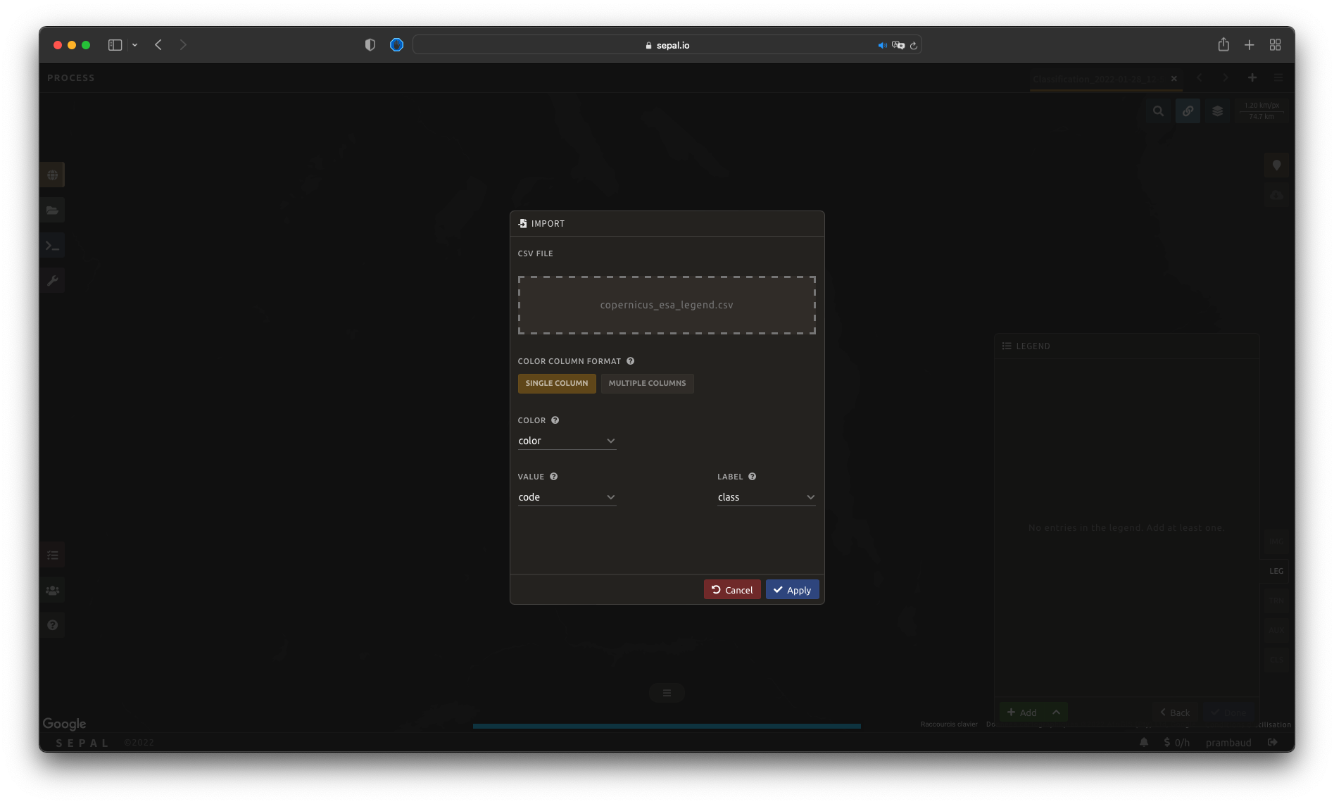
Select Apply to validate your selection. The classes will be added to the legend panel and you’ll be able to modify the legend using the parameters presented in the previous subsection.

Select Done to validate this step.
Every pane should be closed; the colors of the legend should now be displayed at the bottom of the map. No classification is performed, as we didn’t provide any training data. Nevertheless, this step is the last mandatory step for setting parameters. Training data can be added using the on-the-fly training functionality.
Export legend#
Once your legend is validated, select the and then Export as CSV.
A file will be downloaded to your computer named <recipe_name>_legend.csv, which will contain the legend information in the following format:
color,value,label
#006400,10,Tree cover
...
Training data setup#
Two inputs are required to create the classification output:
pixel values (e.g. bands) to classify; and
training data to set up the classification model.
This menu will help the user manage the training data of the model used. To open it, select TRN in the lower-right side of the window.
Import existing training data#
Instead of collecting all data by hand, SEPAL provides numerous ways to include already existing training data into your analysis. The data can be from multiple formats and will be included in the model to improve the quality of the final map.
Note
The imported files can use an extended version of the legend provided in the previous step, but to avoid unexpected behaviour, at least one of the classes of your legend and the provided training data need to match.
Note
If the added training data are outside of the image to classify, they will have no impact on the final result (with the exception of the SEPAL recipe).
To add new data, select Add and choose the type of data to import:

CSV#
By selecting CSV file, SEPAL will request a file from your computer in .csv format. The file needs to include two pieces of information: geographic coordinates and class value.
This can be done using coordinates in EPSG:4326 latitude and longitude, as well as a GeoJSON compatible point object. The file can embed other multiple columns that will not be considered during the analysis.
The following table is compatible with SEPAL:
XCoordinate,YCoordinate,class,class_name,editor_name
32.77189961605467,-11.616264558754402,80,Shrublands,Pierrick rambaud
...
The columns used to define the X (longitude) and Y (latitude) coordinates are manually set up in the pop-up window. Select Next once every column is filled.
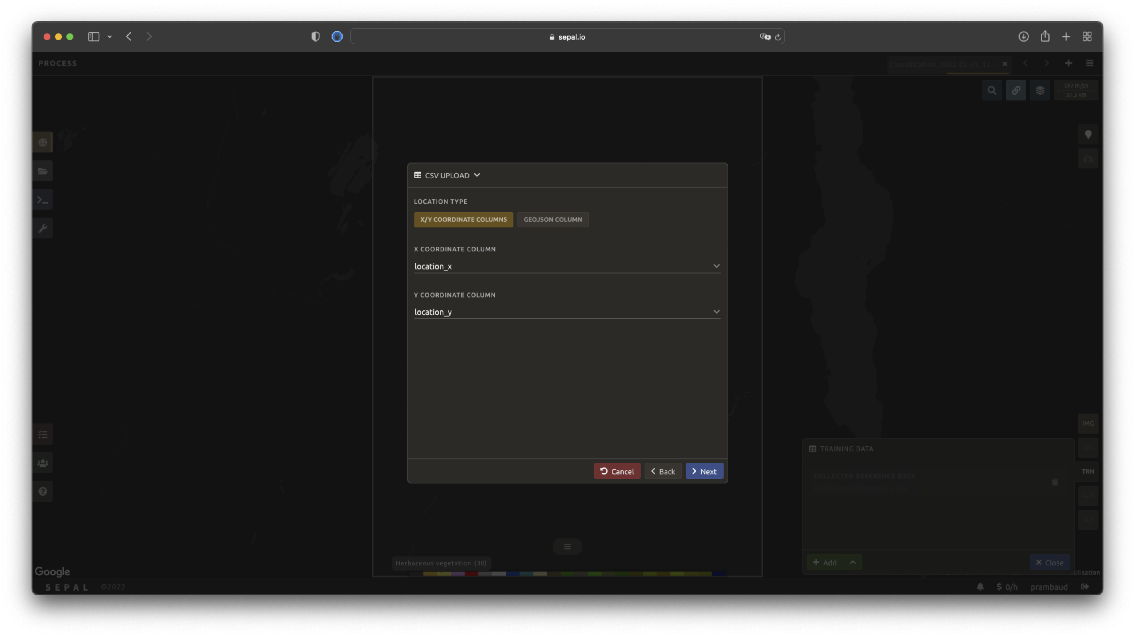
Tip
If your file contains a GeoJSON column instead of coordinates, select GeoJSON column to switch the interface to one column selection.
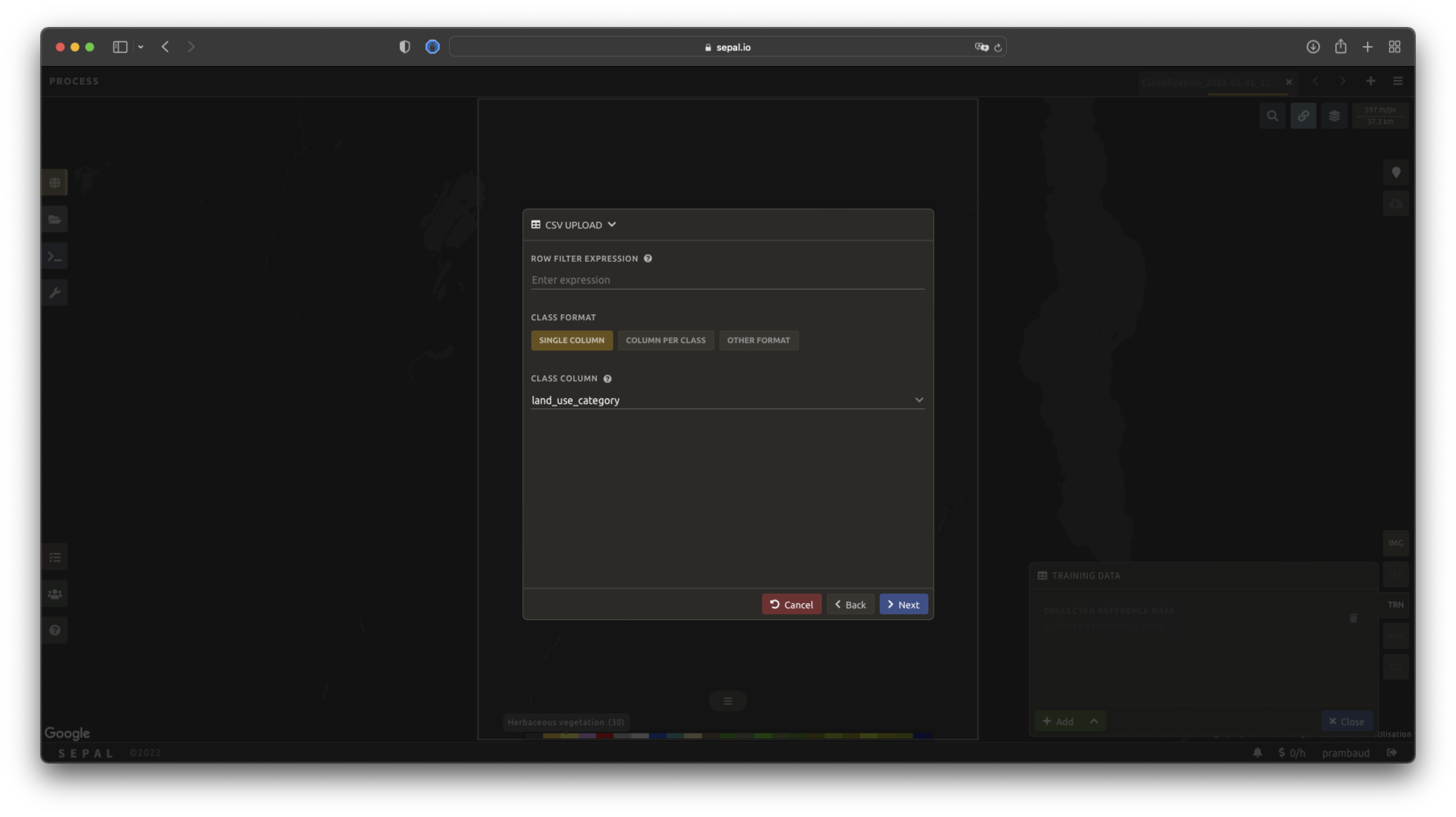
Now that you have set up the coordinates of your points, SEPAL will ask how the class values (not the names) are stored, through the Class format selector:
Single column: all class values are held in a single column — select that column from your file.
Column per class: each class has its own column.
Other format: use this if your data has a different layout.
Tip
Using the Row filter expression field, you can keep only the rows that meet a condition — a JavaScript-like expression, referencing your columns by name, that evaluates to true for the rows to keep (leave it empty to keep all). For example, class == 30 keeps only the rows in class 30, and class == 10 || class == 20 keeps classes 10 and 20.
Select Next to add the data to the model. SEPAL will provide a summary of the classes in the legend of the classification and the number of training points added by your file.
Selecting the Done button will complete the uploading procedure.

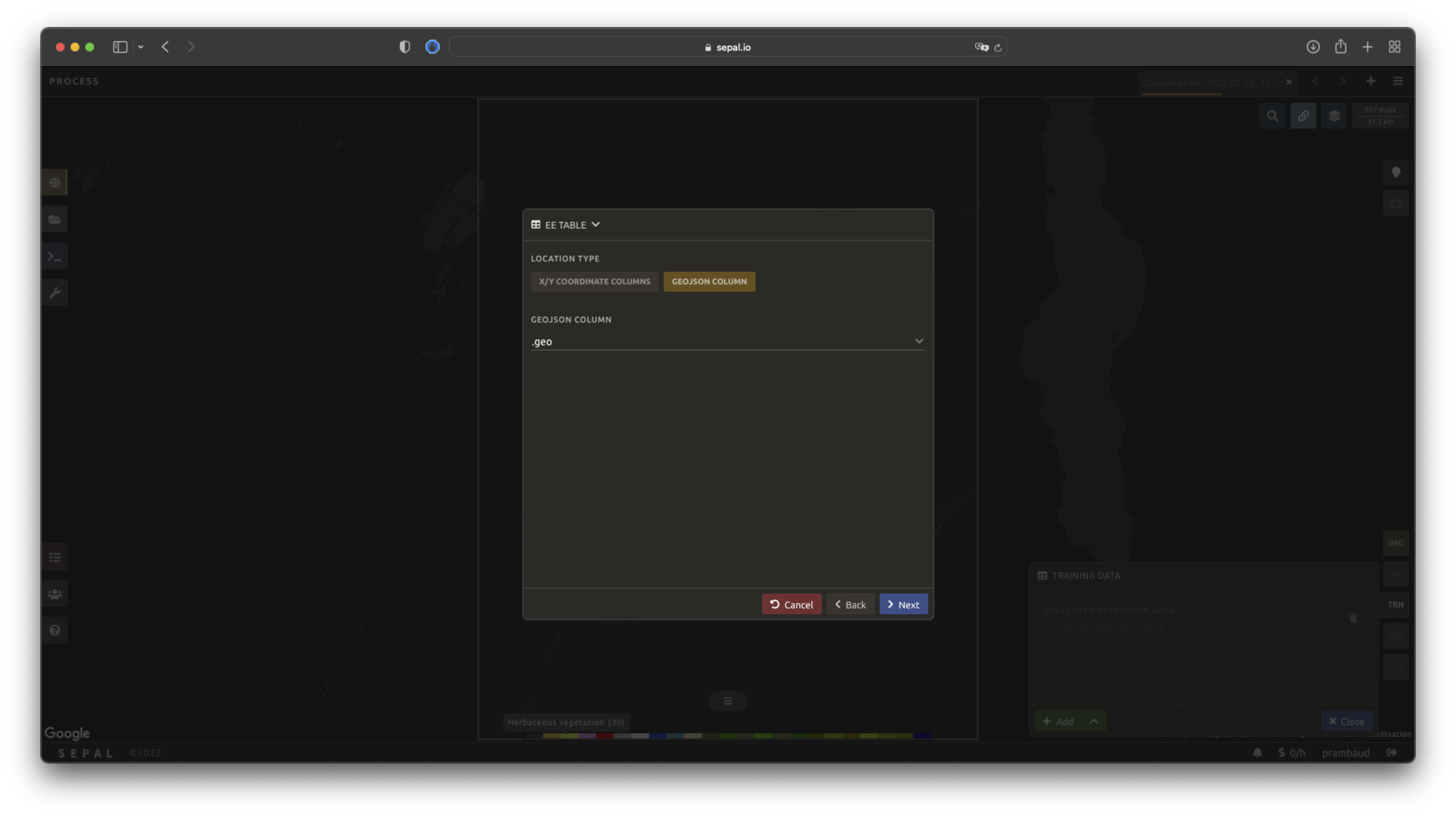
GEE table#
By selecting Earth Engine Table, SEPAL will request a file from your computer in .csv format. The file needs to provide two pieces of information: geographic coordinates and class value.
The process is nearly the same as found in the documentation above discussing .csv tables. The only difference should be the geometry column, as GEE assets usually embed a .geojson column by default. If this column exists, it will be autodetected by SEPAL.
For the other steps, please reproduce what was presented in the .csv section above.
Note
To build the documentation example, use this public asset: projects/sepal-cookbook/assets/classification/zmb_eastern_esa_2012_2021_reference_data.
Sample classification#
Instead of providing dataset points, SEPAL can also extract reference data from an already existing classification – which is a good way to improve an already existing classification system using an image with a better resolution.
To sample data, SEPAL will randomly select a number of points in each class and extract the class value using the provided resolution.
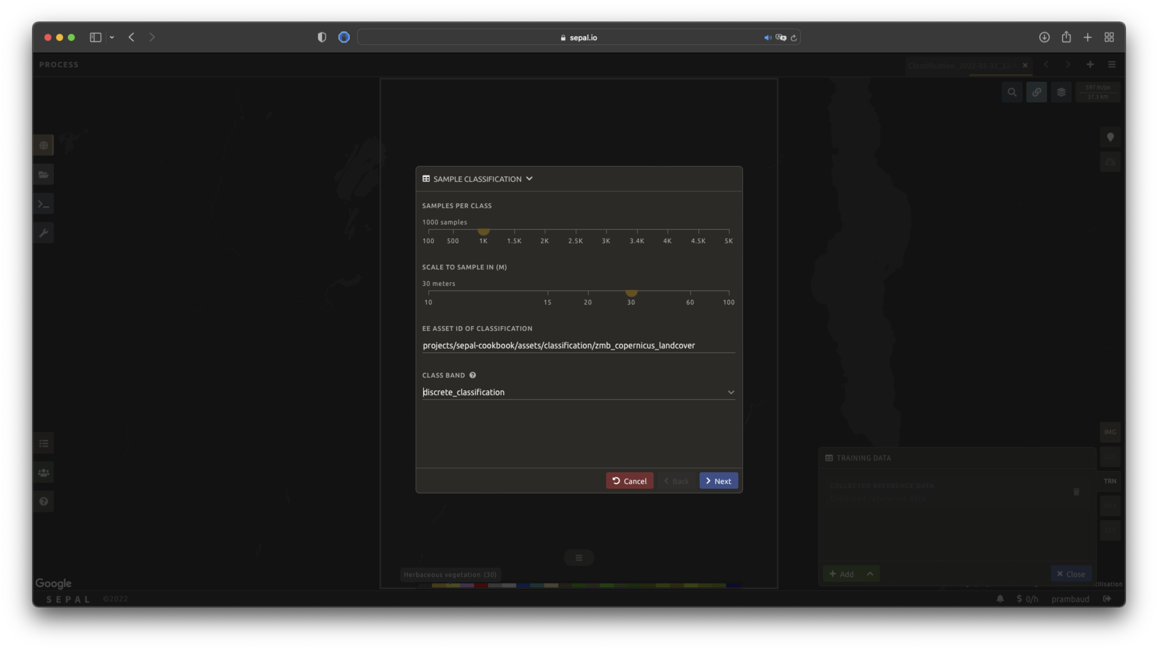
Start by selecting Sample classification in the opened pop-up window, where all of the parameters can be set:
Samples per class: the number of samples per class of the provided image. The more samples you request, the more accurate the model will be (if too many samples are selected, on-the-fly visualization will never render). The default is
100, but you can pick other preset values, such as the1000used in this example.Scale to sample in: the scale used to create the sample in the provided image (it should match the image to classify resolution; default to:
30 m).Image source: choose whether to sample from an existing EE Asset or a saved Recipe.
EE asset ID of classification: when EE Asset is selected, the ID of the classification to sample (it should be an
ee.Imageaccessible to the user). When Recipe is selected instead, choose one of your saved classification recipes to sample.Class band: The class to use for classification value (the dropdown menu will be filled with the bands found in the provided asset or recipe).
Note
When all of the parameters are selected, it can take time, as SEPAL builds the sampling values on the fly. They will only be displayed once the sampling is validated.
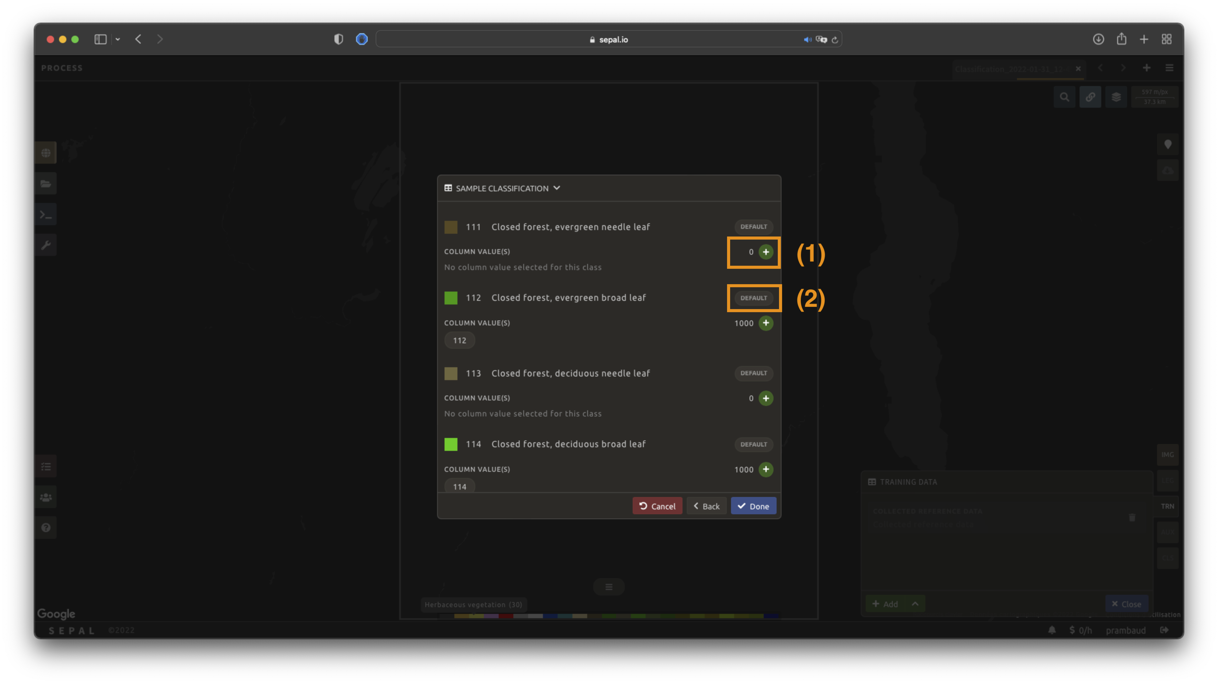
Select Next to display the sampling summary. In this pane, SEPAL displays each class of the legend (as defined in the previous subsection) and the number of samples created for it.
Each class shows its sample count next to a green button — use it to change the number of samples for that class. By default, SEPAL ignores the samples with a Null value; select Default on any class so that these points end up in the default class instead of being ignored.
SEPAL recipe#
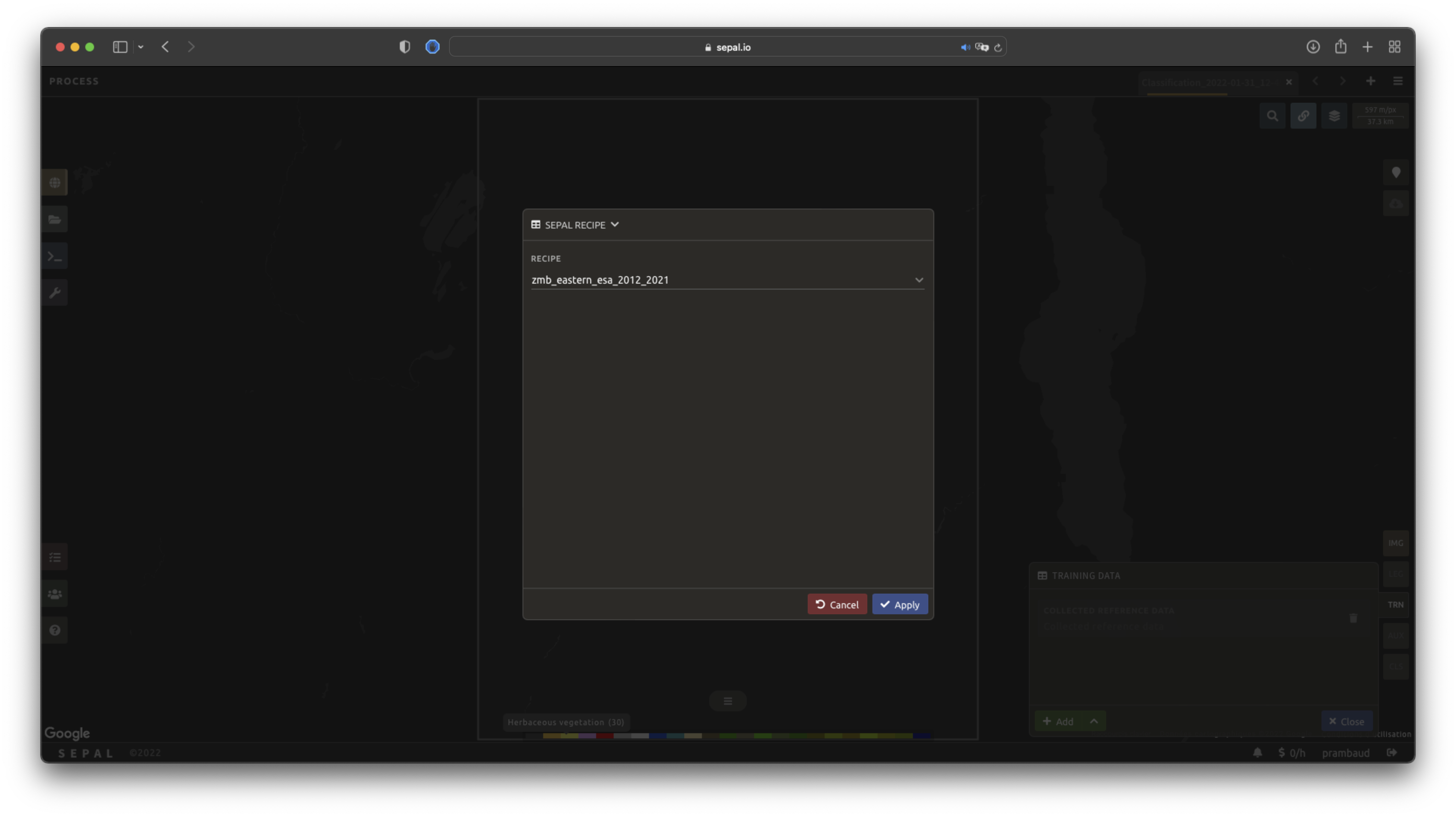
SEPAL is also able to directly apply a model built in another recipe as training data. In this case, we are not importing the points, but all of the model from the external recipe. It will not add points to the map. It’s useful when the same classification needs to be applied on the same area for multiple years. The classification work can be carried out only in the first year and then applied recursively on all the others.
Select Saved SEPAL recipe to open the pop-up window. In the dropdown menu, select one of the recipes saved in your SEPAL account.
Note
The imported recipe needs to be a Classification recipe. If none are found, the dropdown menu will be empty.
This recipe cannot come from another SEPAL account.
Collect Earth Online#
SEPAL can import training data you have collected in a Collect Earth Online (CEO) project directly, without exporting and re-uploading a file. Select Collect Earth Online to open the panel.
Connect to your CEO account
The panel starts as Disconnected from CEO.
Select Connect to open the Collect Earth Online Authentication window, enter your CEO Email and CEO Password, and select Connect again.
Note
Your credentials are never stored on SEPAL servers. When your SEPAL session ends, the CEO connection is terminated automatically. You can also select Disconnect at any time to end it manually.
Select the institution and project
Once connected (You are connected to CEO), fill in:
Institution: the CEO institution to pull data from. Only institutions where you are both a member and an admin are listed.
Project: the project within that institution whose collected data you want to use.
Data type: whether to import the project’s Plot (aggregated plot) data or its Sample data.
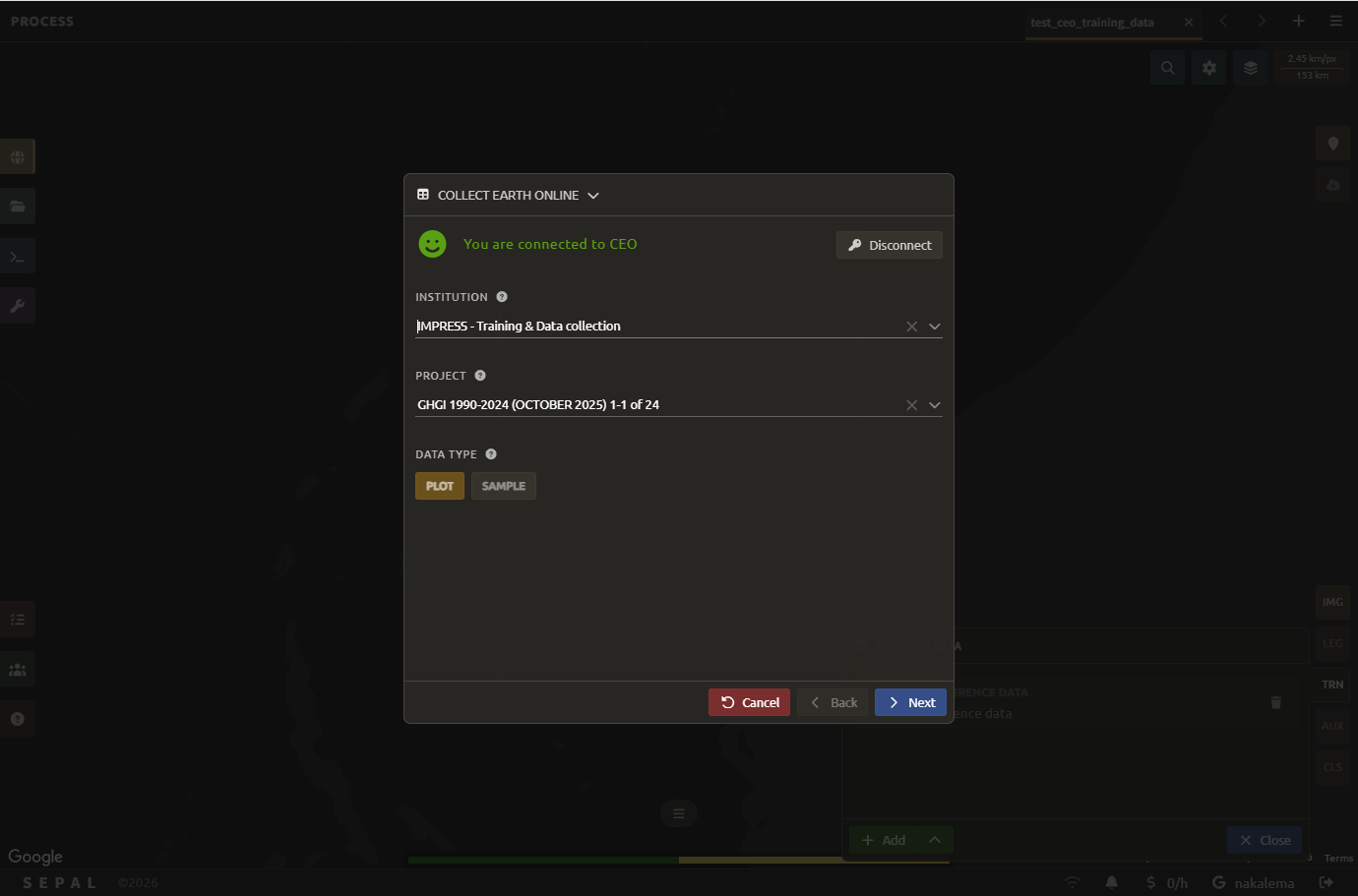
SEPAL then loads the collected data, ready to be mapped to your legend in the next two steps.
Set the location
SEPAL reads the point locations from the data and pre-fills the Location type (X/Y coordinate columns or GeoJSON column) together with the matching coordinate columns. These are detected automatically from the CEO data, so you can usually confirm them as they are.
Set the class format
Tell SEPAL how the class values are stored in the CEO data, through the Class format selector:
Single column: all class values are held in a single column.
Column per class: each class has its own column. CEO data is mostly organized this way.
Other format: use this if your reference data has a different layout.
SEPAL pre-selects the format based on the chosen data type, but you can change it.
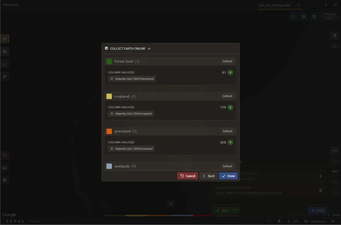
Select Next to reach the class summary, which lists each legend class. For every class, select the button to choose the column that corresponds to it, then select Done to add the reference data to the model.
Manage collected reference data#
Collected reference data are the points you add directly on the map with the on-the-fly training tool, described in the On-the-fly training section. Each point pairs a set of coordinates with a class value. Select the button — to the right of the Add button in the TRN tab — to manage them:
Export reference data to CSV: download a
<recipe_name>_reference_data.csvfile to share your points with others. It will embed all of the gathered point data using the following convention:XCoordinate,YCoordinate,class 32.77189961605467,-11.616264558754402,80 ...
Clear collected reference data: remove every collected point from the analysis.
Tip
A confirmation pop-up prevents you from accidentally deleting everything.
Use auxiliary datasets#
Some information that could be useful to the classification model is not always included in your image bands. A common example is Elevation. In order to improve the quality of the classification, SEPAL can provide some extra datasets to add auxiliary bands to the classification model.
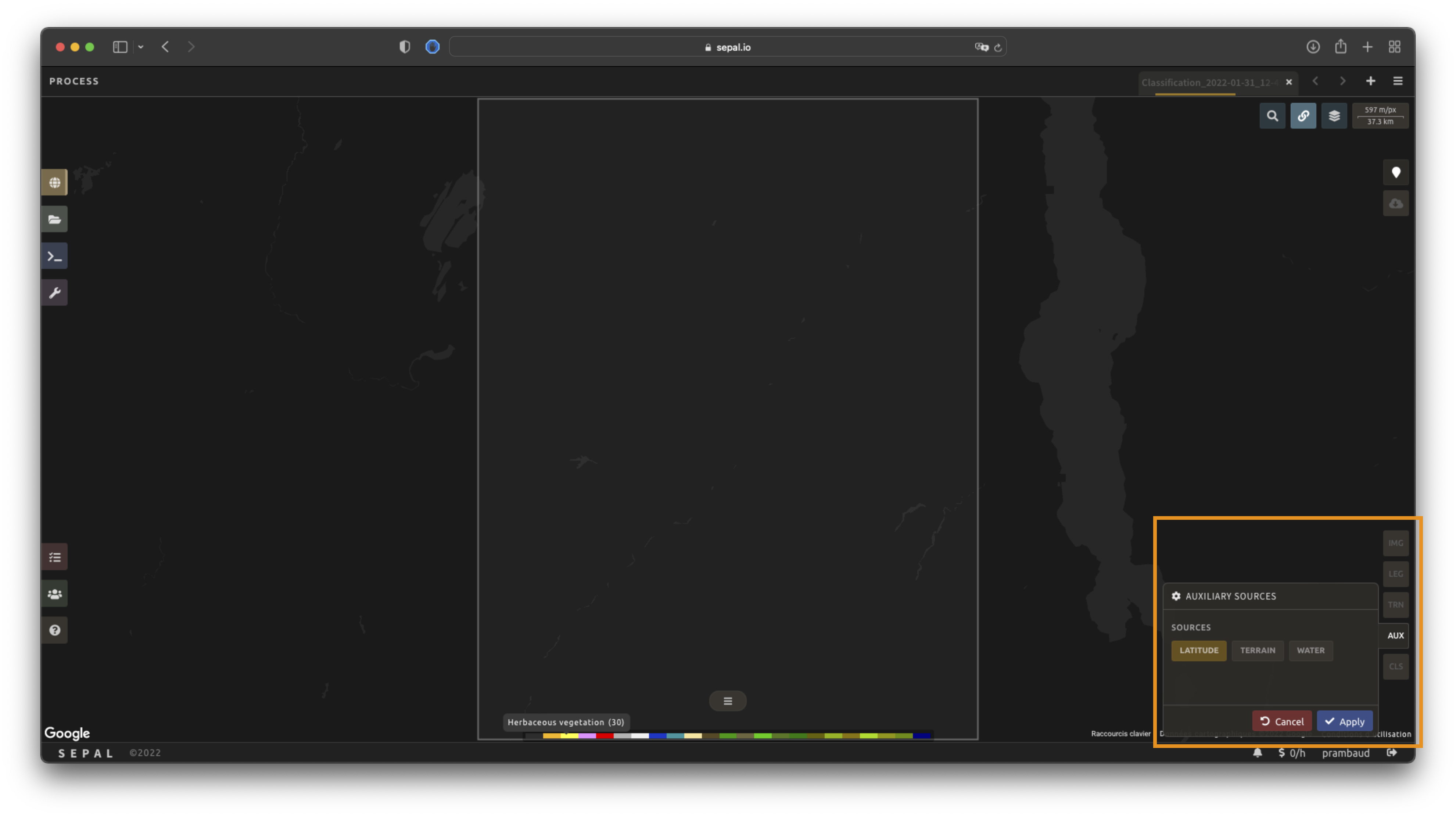
Select AUX to open the Auxiliaries tab. Three sources are currently implemented in the platform (any number of them can be selected):
Latitude: On-the-fly latitude dataset built from the coordinates of each pixel’s center.
Terrain: From the NASA SRTM Digital Elevation 30 m dataset, SEPAL will use the
Elevation,SlopeandAspectbands. It will also add anEastnessandNorthnessband derived fromAspect.Water: From the JRC Global Surface Water Mapping Layers, v1.3 dataset, SEPAL will add the following bands:
occurrence,change_abs,change_norm,seasonality,max_extent,water_occurrence,water_change_abs,water_change_norm,water_seasonalityandwater_max_extent.
Classifier configuration#
Note
Customizing the classifier is a section designed for advanced users. Make sure that you thoroughly understand how the classifier you’re using works before changing its parameters.
Note
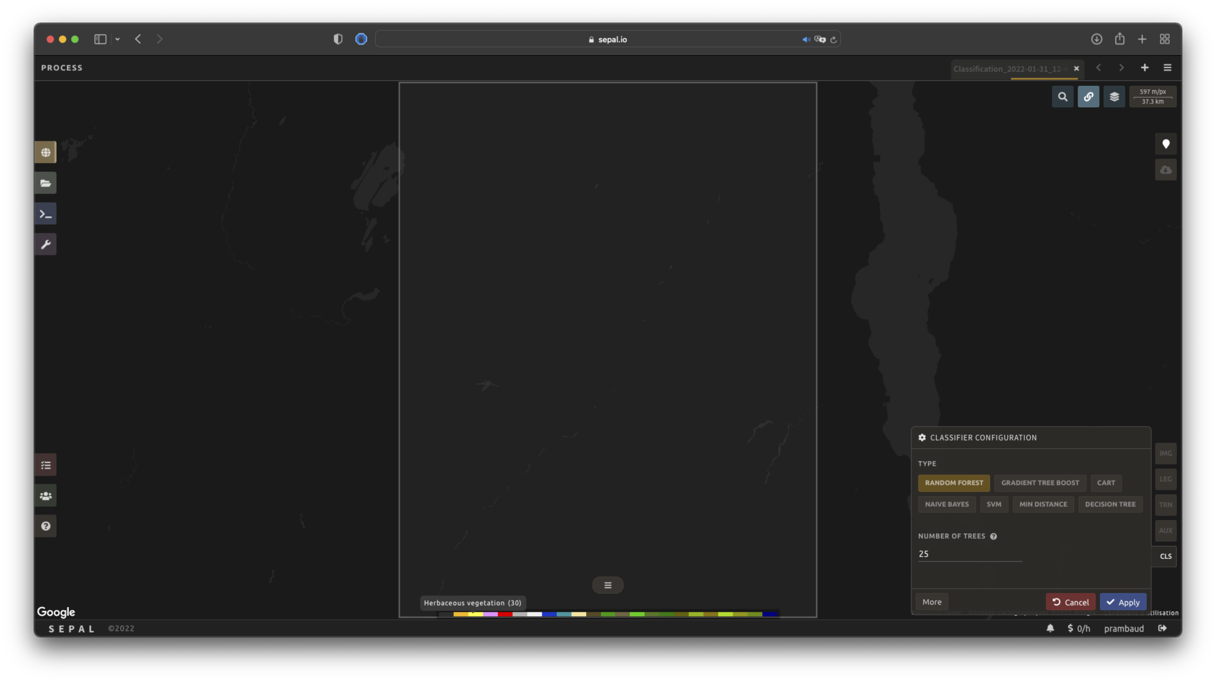
The default value is a Random Forest classifier using 25 trees.
The Classification tool used in SEPAL is based on the Smile - Statistical Machine Intelligence and Learning Engine Javascript library (refer to their documentation for specific descriptions of each model).
Select CLS to open the Classification parameter menu. SEPAL supports seven classifiers:
Random Forest
Gradient tree boost
Cart
Naive bayes
SVM
Min distance
Decision tree
For each of them, the workflow is the same:
Select the classifier by clicking on the corresponding name. SEPAL will display some of the parameters available.
Select More on the lower-left side of the panel to fully customize your classifier. The classification results will be updated on the fly.

Refine the classification#
Note
This process requires a good understanding of the Visualization feature of SEPAL (see Visualization in SEPAL for more information).
Once all of the parameters are set, you can refine the classification directly on the map: set up the view, add or edit training points on the fly, and check the model’s confidence.
Set up the view#
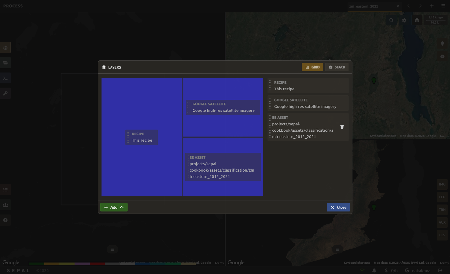
In order to improve the classification, one must set up the view to display all of the information; you choose what the map shows from the Layers panel. Select the layers-to-show icon in the top-right of the screen to open the panel, then:
Pick a layout mode — Grid to split the map into several panes side by side, or Stack to overlay the layers in a single pane.
Drag and drop each layer onto a position (centre, a side, or a corner) to choose where it appears; drag it between positions to rearrange it, or off the areas to remove it.
If the layer you need is not already in the panel, select Add to add a source: Add a SEPAL recipe, Add an Earth Engine asset, or Add a Planet account.
With your layers arranged, the map displays them together so you can compare them while adding training data.
In the following image, we displayed:
The current recipe (1) using the class colors in categorical mode.
The current image (what you are classifying) (2) using the NIR,RED,SWIR1 band combination.
The extra visual dataset NICFI Planet Lab data (3) from 2021.
The number (4) indicates a cluster of existing training points. Zoom in and they will be displayed as markers using the color of the class they mark (5).
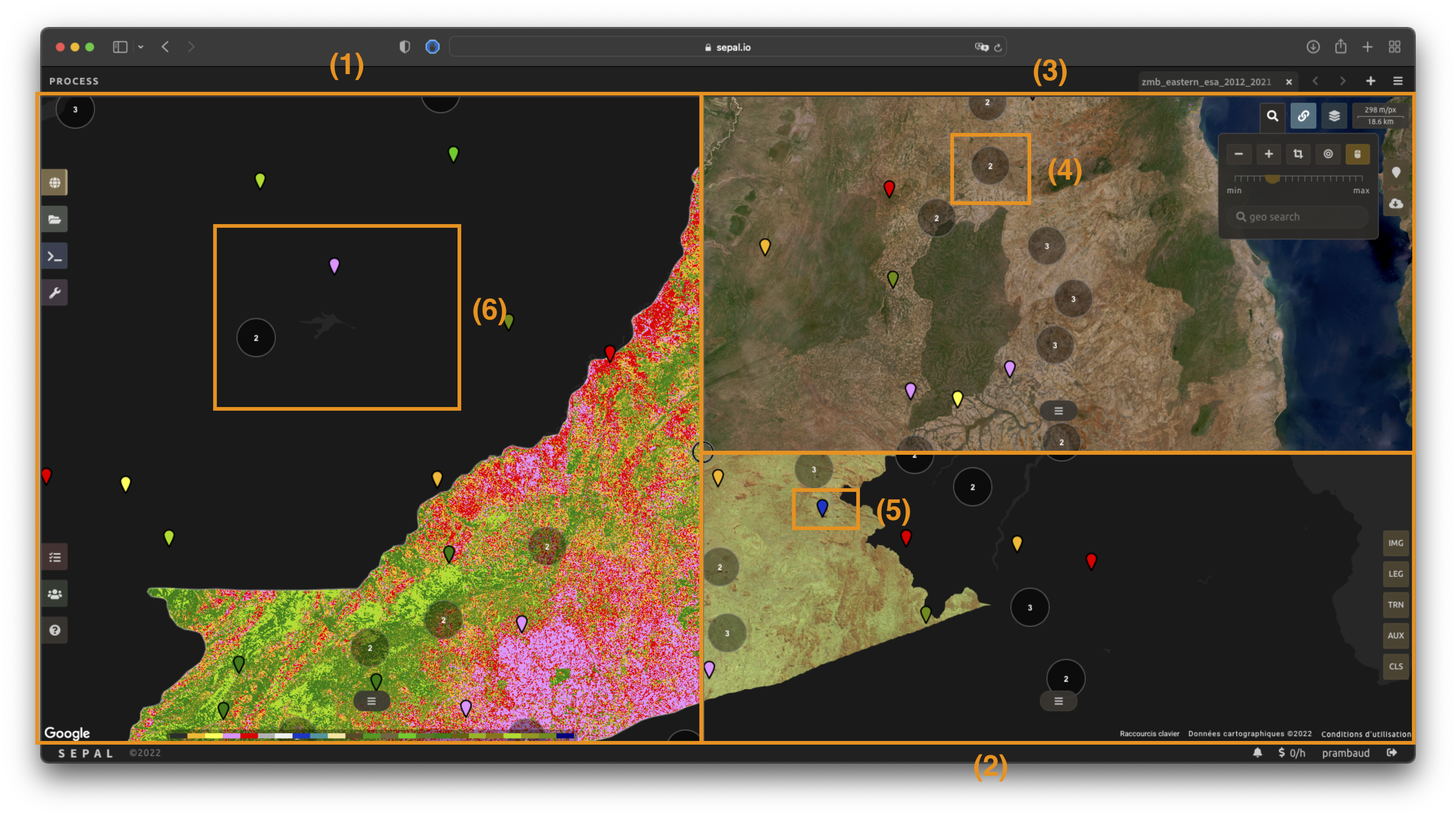
Important
This initial classification has been set using sampled data. Since they are sampled from a larger image, some are out of the image. They will have no impact on the classification as they are applied to masked pixels (6).
On-the-fly training#
You are free to add extra training data in the web interface; each new point is added to the final model, improving the quality of the classification.
Select points#
To start adding points, open the training interface by selecting in the upper right of the screen (1). Once selected, the background color becomes darker and the pointer of the mouse becomes a .
The process to add new training data is as follows:
Click on the map to select a point: You can click in any of the panes (not restricted to the Recipe pane), but to be useful, the point needs to be within the border of the AOI. If it’s not already the case, the Class selection panel will appear in the upper right of the window (2).
Select the class value: The previous class value is preselected, but you can change it to any other class value from the defined legend. The legend is displayed as
<legend_classname> (<legend_value>).
You can now click elsewhere on the map to add another point. If you are satisfied with the classification, select Close (3) and select again to stop editing the points. Every time a new point is added, the Classification map is recomputed and rendered on the left side.
Modify existing points#
To modify existing points, select the to open the Point editing interface. Then:
Select a point: To select a point, click on an existing marker. It will appear bolder than the others. If it’s not already the case, the Class selection pane will appear in the upper right.
Change the class value: The point class will be selected in the Editing menu with a . Select any other class value to change it.
Check the validity#
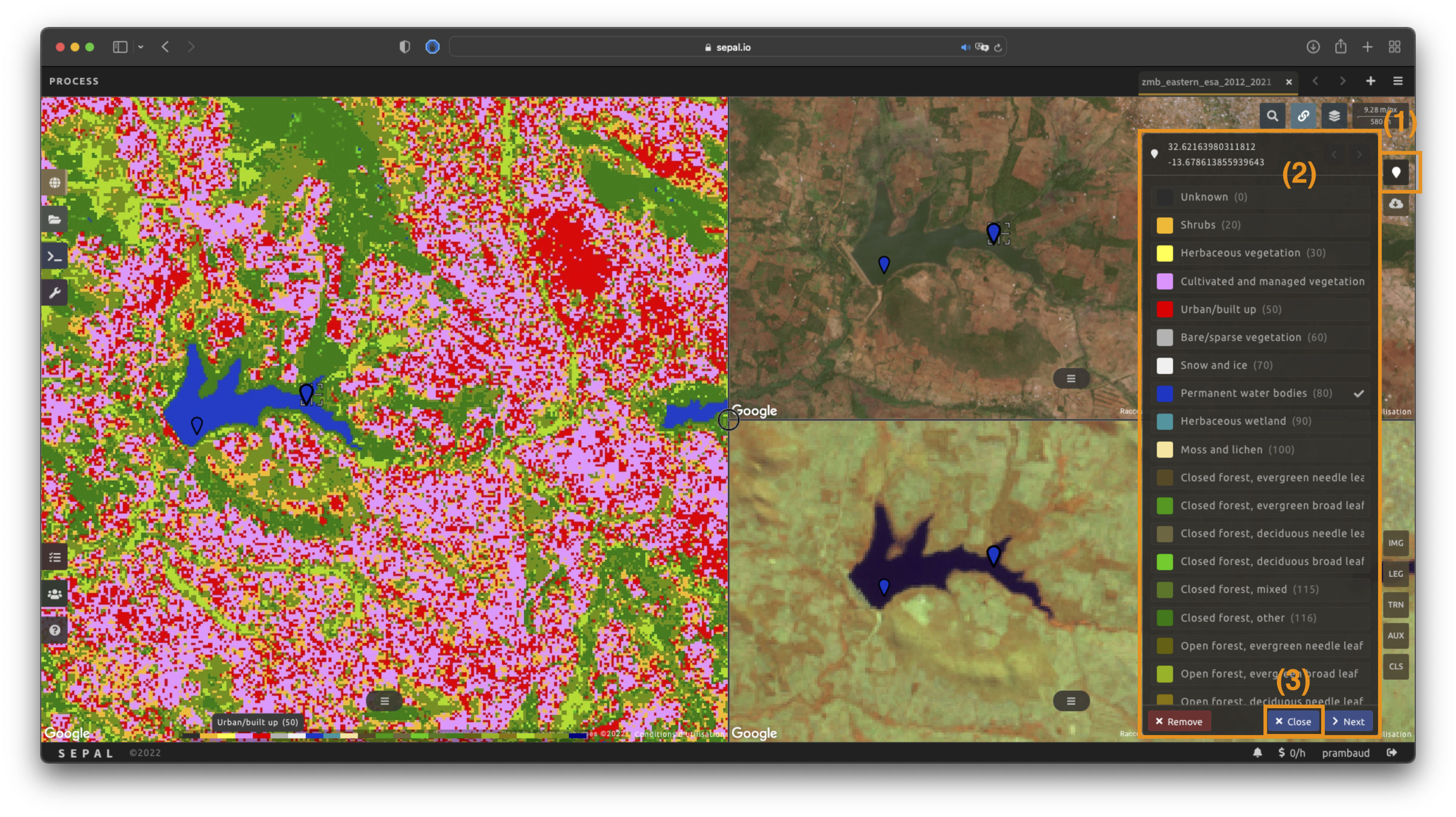
SEPAL embeds information to help the user understand if the amount of training data is sufficient to produce an accurate classification model. In the Recipe window, select the button at the bottom centre of the map to open the layer’s options, then change the Bands selector to Class probability.
The user now sees the probability of the model (i.e. the confidence level of the output class for each pixel).
If the value is high (> 80 percent), then the pixel can be considered valid; if the value is low (< 80 percent), the model needs more training data or extra bands to improve the analysis.
In the example image, the lake is classified as a permanent water body with a confidence of 65 percent, which is higher than the rest of the vegetation around it.

This analysis can also be conducted class-by-class using the built-in <class_name> % bands. Select the one corresponding to the class you want to assess (see the following image) and you’ll get the percentage of confidence for each pixel to be in the sub-mentioned class.

Export#
Important
You cannot export a recipe as an asset or a .tif file without a small computation quota. If you are a new user, see Manage your resources.
Start download#
Selecting the tab will open the Retrieve pane where you can select the exportation parameters.
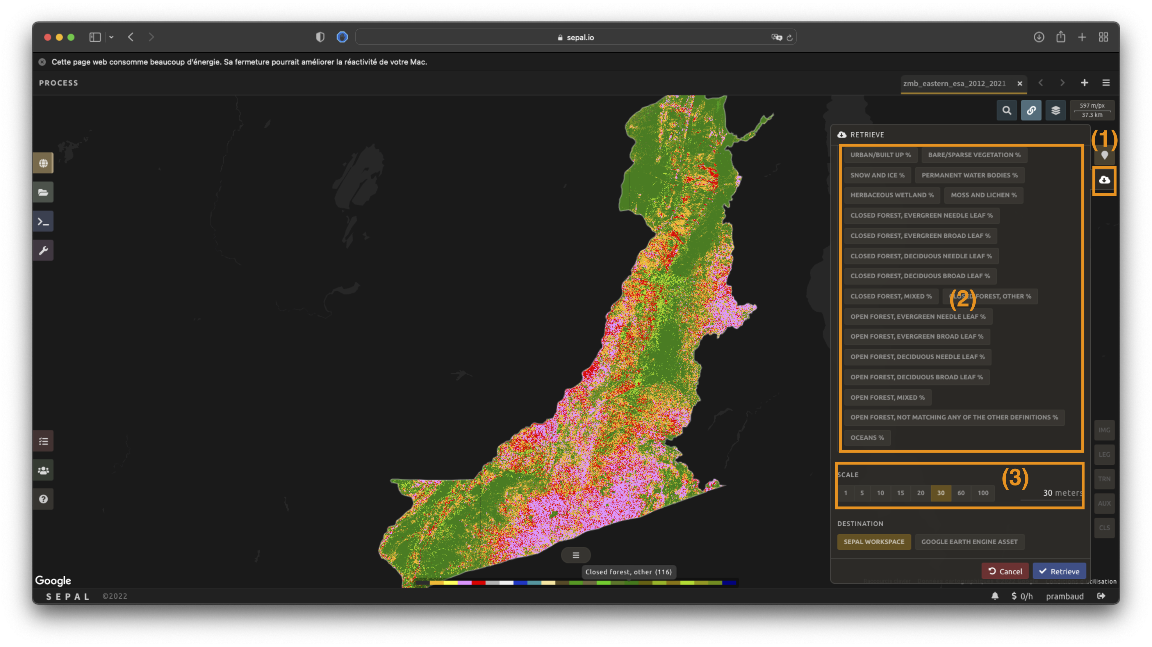
Bands#
You need to select the band(s) to export. There is no maximum number of bands, but exporting useless bands will only increase the size and time of the output. The available bands include the classified Class band, the Class probability band, and the per-class confidence (<class_name> %) bands.
Scale#
You can set a custom scale for exportation by selecting a value in metres (m) (note that requesting a smaller resolution than the images’ native resolution will not improve the quality of the output – just its size – keep in mind that the native resolution of Sentinel data is 10 m, while Landsat is 30 m).
Destination#
Choose a single destination for the export:
SEPAL workspace: the image is written to your SEPAL files in
.tifformat (by default in theDownloadsfolder).Google Earth Engine asset: the image is exported to your GEE account as an asset. You can export it either as a single Image or as an Image collection (tiled, which is better suited to large exports), and set its sharing to Private or Public.
Google Drive: the image is exported to the Google Drive of the connected Google account.
Note
The Google Earth Engine asset and Google Drive destinations are only displayed when a Google account is connected to SEPAL. If they are missing, please refer to Connect SEPAL to GEE.
Select Retrieve to start the export process.
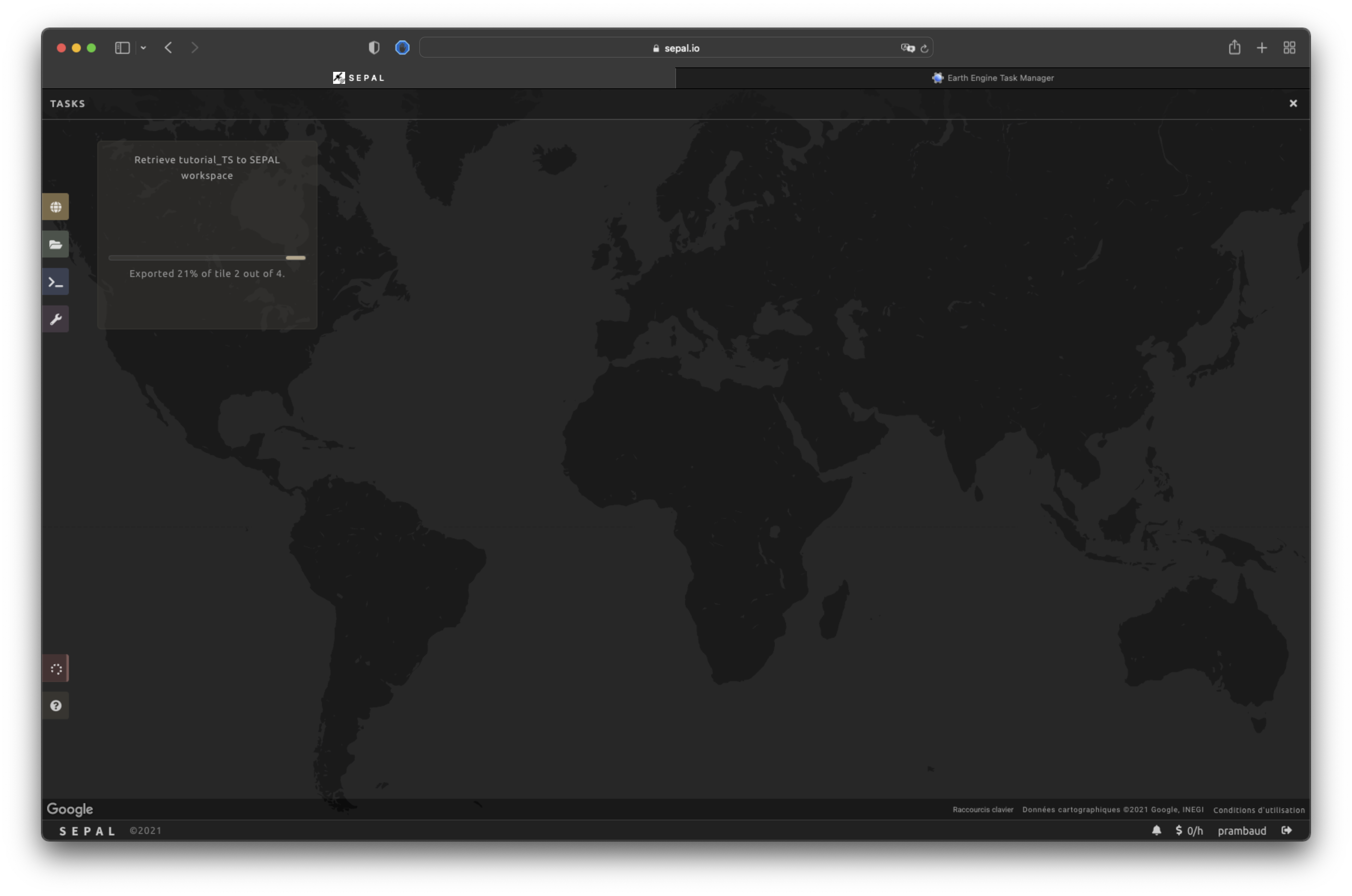
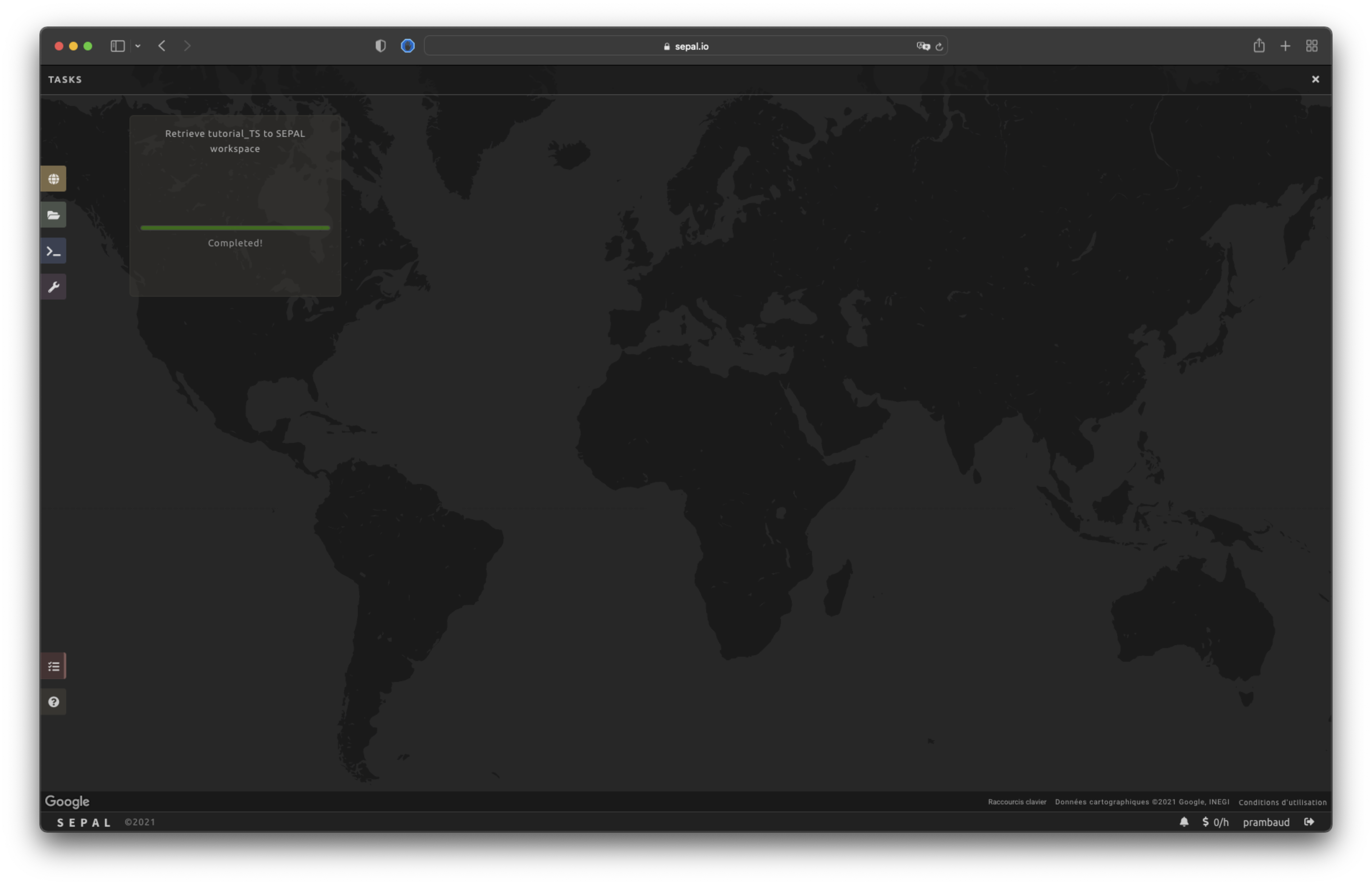
Exportation status#
By going to the Tasks tab (in the lower-left corner using the or buttons, depending on the loading status), you will see the list of different loading tasks.
The interface will provide you with information about the task progress and display an error if the exportation has failed. If you are unsatisfied with the way we present information, the task can also be monitored using the GEE task manager.
Tip
This operation is running between GEE and SEPAL servers in the background. You can close the SEPAL page without ending the process.
When the task is finished, the frame will be displayed in green, as shown in the second image below.
Access#
Once the download process is done, you can access the data in your SEPAL folders. The data will be stored in the Downloads folder using the following format:
.
└── downloads/
    └── <CLASSIF name>/
        ├── <CLASSIF name>_<gee tile id>.tif
        ├── <CLASSIF name>_<gee tile id>.tif
        ├── ...
        ├── <CLASSIF name>_<gee tile id>.tif
        └── <CLASSIF name>_<gee tile id>.vrt
Note
Understanding how images are stored in an optical mosaic is only required if you want to manually use them. The SEPAL applications are bound to this tiling system and can digest this information for you.
The data are stored in a folder using the name of the optical mosaic as it was created in the first section of this article. As the data are spatially too big to be exported at once, they are divided into smaller pieces and brought back together in a <MO name>_<gee tile id>.vrt file.
Tip
The full folder with a consistent tree folder is required to read the .vrt.