Direct drivers assessment

Map disturbances and quantify the contribution of associated direct drivers to assess deforestation and forest degradation trends, and their associated current and historical direct drivers

Note

This article was produced in the framework of the global project, Assessment of deforestation and forest degradation and related direct drivers using SEPAL, supported by the Central African Forest Initiative (CAFI).

The Deforestation and Degradation Drivers (DDD) project is a global methodology developed and piloted in Central Africa. While the Congo Basin is used as an example, the methodology can be applied to any geographic area.

Background

Deforestation and forest degradation are complex processes that have many underlying causes. A comprehensive understanding of forest conversion to other land uses is instrumental for the development of policies and actions aiming to reduce the loss of forests and associated carbon emissions. It is important to understand recurring patterns and correlations that can help countries tailor their efforts toward reducing forest loss.

The causes of deforestation and forest degradation vary both regionally and temporally (Curtis, 2018). Different studies refer to agricultural expansion (cropland and pasture) as the largest direct cause of global deforestation (FAO, 2022; Gibbs, 2010; Hosonuma, 2012; Kissinger, 2012; Sandker, 2017). Commercial agriculture is estimated to be responsible for around 70–90 percent of worldwide deforestation. In Africa, both commercial and subsistence agriculture may account for similar importance in terms of forest loss, while fuelwood collection, charcoal production, and livestock grazing in forests (to a lesser extent), are the most important drivers of degradation.

However, these studies (as well as existing national studies on the drivers of deforestation and forest degradation in Central Africa) are generally based on data acquired up to 2014 and do not consider the recent trends in observed tree cover loss. They also do not take into account the importance of the spatial fragmentation of forests and the role played by degradation induced by forest exploitation (Molinario, 2015). Furthermore, they simplify causes of deforestation into a single driver, which does not adequately reflect the complex local context and interacting causes – decisions that lead to anthropogenic forest disturbance at local levels (Ferrer-velasco, 2020).

These recent trends and the lack of updated studies result in little consensus on the main drivers and agents of forest change at regional levels. There is a pressing need to systematically quantify the direct causes of deforestation and degradation via a systematic and comprehensive approach. An updated assessment should provide validated evidence on the role and weight of different drivers of forest loss and support decision-making to address related challenges. A spatially explicit approach should also facilitate the assessment of the efficiency of policies and actions in different contexts. Improved spatial data on deforestation and forest degradation, as well as an improved understanding of the drivers, will support land-use planning approaches in two pilot areas where the regional analysis indicated a clear opportunity for supporting land-use planning and decision-making.

In this context, the Food and Agriculture Organization of the United Nations (FAO) has developed a robust methodology to assess the recent trends and drivers of deforestation and forest degradation. It involves collaborative approaches in which national experts, research institutes and civil society work together and compile resources and data to reach a common view on the current and future causes and drivers of anthropogenic forest disturbances. These tools generate improved information for decision-making and land-use planning in relevant management contexts.

FAO, in partnership with CAFI, as well as a coalition of donor and partner countries, have developed a standard, global, large-scale methodology to assess forest dynamics using cloud-computing solutions and open-source tools. The approach maps disturbances (both deforestation and degradation) and quantifies the contribution of multiple associated direct drivers. The methodology is used to assess deforestation and forest degradation trends, and their associated current and historical direct drivers in six Central African countries as part of an international effort to mitigate climate change, support the Sustainable Development Goals (SDGs), and protect biodiversity. The project builds on a collaborative approach, in which national experts, global research institutes, and civil society work together, as well as compile resources and data, to provide technical evidence and reach a common view on the current and historical trends, as well as direct drivers of forest disturbances.

Definitions

A robust methodology uses consistent definitions. The following terms and definitions are applied throughout the workflow.

Area of interest

The pilot study area includes the national boundaries of the six Congo Basin countries: Cameroon, the Central African Republic, the Democratic Republic of the Congo, Equatorial Guinea, Gabon, and the Republic of the Congo.

Because of consistency issues between border datasets (at the national, regional and/or global levels), it was decided to take one global dataset: Large Scale International Boundaries (LSIB), from the Department of State of the United States of America.

Forest definitions

There are a total of four different national forest definitions in the six countries of the study region. These are applied at country level using information on canopy height, tree cover and pixel area.

Scale	Source	Date	Minimum mapping unit (ha)	Tree height (m)	Canopy cover (%)	Comment
Cameroon	REDD+ National Strategy (MINEP, 2008)	2018	0.5	3	10%	Exclusion of monospecific agro-industrial plantations with a purely economic vocation and using mainly agricultural management techniques; are always considered as forest the areas subjected to natural disturbances which are likely to recover their past status.
Central African Republic	FRA	2020	0.5	5	10%
Democratic Republic of the Congo	FREL 2018 (Ministère de l’Environnement et Développemnt Durable, 2018)	2018	0.5	3	30%	A canopy cover criterion of around 50% for an area of 0.09 ha was used during the interpretation of the samples.
Gabon	Sannier et al., 2016	2020	0.5	5	30%	Functional definition used by national monitoring system (AGEOS).
Republic of the Congo	FREL (Coordination Nationale REDD, 2017)	2017	0.5	5	30%	Exclusion of agricultural activities, in particular palm groves in production.

Regional land cover

The baseline map for the regional forest cover was first derived from a common classification system that was validated by the project technical committee and included land cover classes referenced in the national system. The land cover classification was also published in the FAO Land Cover Registry.

Note

In Cameroon and the Central African Republic, shrub savannahs were identified as forest, in adherence to the national forest definition referencing >10% tree cover.

Code	Forest/non-forest	English	French	Spanish	Description
1	Forest	Dense forest	Forêt Dense	Bosque denso	Dense humid primary evergreen forest on terra firme, >60% tree cover
2	Forest	Dense dry forest	Forêt Dense Sèche	Bosque denso seco	Dense dry forest, >60% tree cover, with dry seasons
3	Forest	Secondary forest	Forêt Secondaire	Bosque secundario	Open forest, 30–60% tree cover, degraded or secondary
4	Forest	Dry open forest	Forêt Claire Sèche	Bosque claro Seco	Dry open forest, 30–60% tree cover, with dry seasons
5	Forest	Sub-montane forest	Forêt Sub-Montagnarde	Bosque sub-montañoso	Forest >30% tree cover, 1100-1750 m altitude
6	Forest	Montane forest	Forêt Montagnarde	Bosque montañoso	Forest >30% tree cover >1750 m altitude
7	Forest	Mangrove	Mangrove	Manglar	Forest >30% tree cover on saline waterlogged soils
8	Forest	Swamp forest	Forêt Marécageuse	Bosque pantanoso	Swamp mixed foret, >30% tree cover, flooded > 9 months
9	Forest	Gallery forest	Forêt Galerie	Bosque en galería	Riparian forest in valleys or along river edges
10	Forest	Mature forest plantation	Plantation Forestière Mature	Plantación forestal madura	Tree cover >15%, cultivated or managed
11	Forest	Woodland savannah	Savane Arborée	Sabana arbórea	Woodland savannah 15-30%, tree cover > national forest definition
12	Forest*	Shrubland savannah	Savane Arbustive	Sabana arbustiva	Shrubland savannah >15% shrub cover > national forest definition
13	Non-forest	Herbaceous savannah	Savane Herbacée	Sabana herbácea	Grassland savannah <15% tree cover
14	Non-forest	Aquatic grassland	Prairie Aquatique	Pradera acuática	Regularly flooded grassland
15	Non-forest	Bare land	Sols Nus - Végétation Éparse	Suelo desnudo-Vegetación escasa	<15% vegetation cover
16	Non-forest	Cultivated areas	Terres Cultivées	Tierras cultivadas	Cultivated vegetation >15% vegetation cover
17	Non-forest	Developed areas	Zones Bâties	Zonas edifiadas	Human dominated and artificial surfaces
18	Non-forest	Water	Eau	Agua	Water > 50%
19	Non-forest	Shrubland savannah	Savane Arbustive	Sabana arbustiva	Shrubland savannah >15% tree cover < national forest definition

Definitions of deforestation and degradation

In order to properly discern between deforestation and degradation, we require specific and operational definitions that can be identified from satellite image analysis.

Deforestation	Degradation
Permanent reduction of forest cover below the forest definition	A temporary or permanent reduction of forest cover that remains above the forest definition
Conversion of forest to other land use: agriculture, pasture, mineral exploitation, development, etc.	Includes areas where timber is exploited or trees are removed, and where forest may be expected to regenerate naturally or with silvicultural methods
Excludes areas of planned deforestation, such as timber extraction, or in areas where the forest is expected to regenerate naturally or with silvicultural methods
Includes areas where impacts, overexploitation or environmental conditions prohibit regeneration above the forest cover definition

Example of deforestation

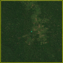
Deforestation is recognizable in images by a permanent change in forest cover. In high-resolution images, we can often see bare ground, felled trees, and sometimes the beginning of agriculture or other driving activities.

Example of degradation

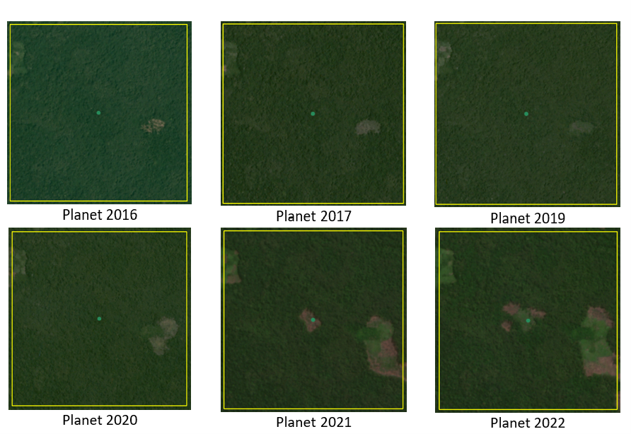
Degradation is more difficult to determine because changes are more subtle (sometimes a few trees removed), and tree cover remains above the national definition. It is therefore necessary to look at the whole time series and make sure that the changes are not deforestation. Degradation is also not the same everywhere and will differ by forest type, as well as environmental and human context.

Date convention

The time period for this pilot study is 2015–2022, with an assessment of changes encompassing 31 December 2015 to 31 December 2022. The year 2015 was used as the baseline, with the detection of annual changes in deforestation and degradation starting in 2016 through 2022. This fits with the availability of Sentinel satellite imagery in 2015 (although incomplete for that year), as well as new monthly high-resolution mosaics available for the tropics from Planet, which are available from 2015 and are used for additional validation.

The following date convention was adopted:

A product for the year YYYY is considered as of 31 December YYYY.

This convention allows a consistent approach to assessing change products. A change map from Year 1 to Year 2 will be consistent with both Year 1 and Year 2 maps. The status of the year takes into account any changes that occurred during the year.

Direct driver definitions

A total of eight direct drivers were defined by their specific characteristics identifiable in high-resolution satellite imagery from Planet.

Driver	Example	Characteristics
Artisanal agriculture		Small-scale agriculture is composed of small, informal, unstructured and irregular agricultural plots covering an area of less than 5 ha. The presence of fires (slash-and-burn agriculture) can be observed; land is often soil cover in various stages of cultivation.
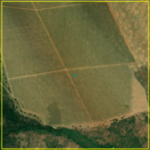
Industrial agriculture		Industrial agriculture is characterized by agricultural areas larger than 5 ha that tend to be homogeneous and often consist of a single crop. In some cases, agriculture may be more varied, consisting of many fields closely packed together. Therefore, large areas consisting of many small fields cultivated at the same time are also considered industrial agriculture under the definition.
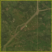
Infrastructure		Roads are visible in images with linear features and are identified as motorized when they are wide enough (5 m) to carry vehicle traffic. Small irregular paths through vegetation are not included. Roads can be large highways or logging trails, and are most often found with other engines, such as villages and mining facilities.
Settlements		Villages and settlements can be hard-roofed or soft-roofed, buildings or huts; they are often accompanied by roads and other drivers such as small-scale agriculture. This engine can be an urban area (left image), or a small isolated village in a forest stand (right image).
Artisanal forestry		Small-scale or artisanal logging is characterized by the selective extraction of trees in an irregular manner, leaving tree cover. These are areas that are not visibly cultivated and are often found in places accessible by small roads or villages.
Industrial forestry		Large-scale or industrial forestry is recognizable by the presence of logging roads, along with selective logging degradation. These roads may be recent or old, and the canopy can quickly cover them, so all years of imagery acquired over the entire study period are evaluated.
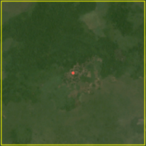
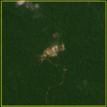
Artisanal mine		Small-scale mining is characterized by muddy clearings and usually ponds or water catchments, and may feature turbid water. Artisanal in nature, the clearings are generally small, isolated, and often located along streams.
Industrial mine		Large-scale mining is characterized by large ponds, open pits and clearings, as well as extensive infrastructure and roads present.

To address the overlapping of drivers in the same location and thus interpret local contexts, our approach identifies archetypes, or common driver combinations which represent realities and processes on the ground. The most common archetype consists of four drivers – artisanal agriculture, artisanal forestry, roads and settlements – which are representative of the agricultural mosaic, or so-called “rural complex”, commonly observed in the region (Molinario, 2020).

The observed combinations of drivers are grouped into thematic classes or archetypes.

Deforestation	Degradation
Rural complex	Artisanal agriculture with roads and settlements, with or without artisanal forestry, and no industrial drivers
Artisanal forestry	Artisanal forestry with or without “other” drivers, or with settlements or roads without any artisanal agriculture
Industrial agriculture	Industrial agriculture and other non-industrial drivers
Industrial forestry	Industrial forestry and other non-industrial drivers
Industrial forestry and agriculture	Industrial forestry and agriculture identified together
Industrial mining	Presence of industrial mining without other industrial drivers
Artisanal mining	No more than two drivers, including artisanal mining; no industrial drivers present
Human infrastructure	Roads, settlements observed alone or together; no other drivers present
Infrastructure-related agriculture	Infrastructure and artisanal agriculture observed together

Methodology

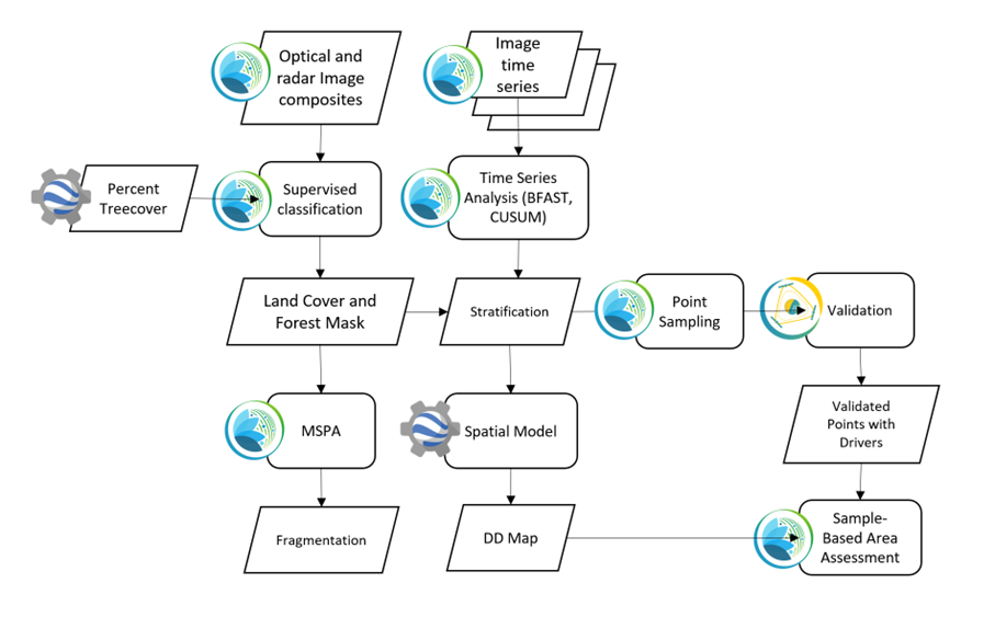
The major components of this methodology include the generation of wall-to-wall geospatial data on forest cover types, changes, and discerning areas of deforestation from degradation for the entire Central African region. Next, these products are validated via visual interpretation; the presence of various direct drivers are identified to evaluate the direct causes of disturbance, and then interpreted in the context of strategic investments for climate change mitigation and support for national efforts for emission reductions.

The methodology uses FAO’s Open Foris Suite of Tools, including the SEPAL platform, for satellite data analysis, as well as Collect Earth Online (CEO) and Google Earth Engine (GEE). The approach analyses dense satellite time series to generate geospatial data on forest changes, which are then validated and interpreted for direct drivers in five major steps:

1. Creating cloud-free mosaics: Processing of optical (Landsat 4, 5, 7 and 8) and radar (Sentinel-1/ALOS PALSAR) satellite images to create mosaics for the classification of wall-to-wall maps of vegetation types, recoded to a binary forest mask (following national forest definitions), and forest fragmentation assessment for the baseline year (2015).

2. Time-series analysis: Processing of optical satellite (Landsat 4, 5, 7 and 8) time series data covering 2012–2020 (2012–2015 is the historical time period; monitoring is from 2016 to 2020), using seasonal models and break-detection algorithms to produce a forest change map for 2015–2020 at the regional scale, identifying areas of both deforestation and degradation.

3. Sample stratification: Stratified random sampling is conducted on the change map from Step 2. Systematic validation for all points identified as change, plus a sample of stable points is conducted in CEO, evaluating land cover types, changes and dates of change, as well as the identification of the presence of direct drivers.

4. Identification of direct drivers: The quantification of direct drivers by forest types and fragmentation class.

Creating cloud-free mosaics

To accurately determine disturbances within forest ecosystems and distinguish from other dynamics occurring in non-forest areas, a baseline forest mask is required. This is achieved by classifying cloud-free image mosaics, which are created using the Optical mosaic and Radar mosaic recipes.

As you can see in this online animation, clouds are persistent in the Congo Basin region. For this reason, we will produce mosaics of optical cloud-free imagery and radar (cloud independent) composites for the best observations of the study region.

Optical cloud-free composite

Multitemporal image mosaics are compiled from data collected over several months or years. Cloud-free pixels from multiple images are integrated into an image with fewer clouds, haze and shadows by using the pixel quality band provided with image metadata.

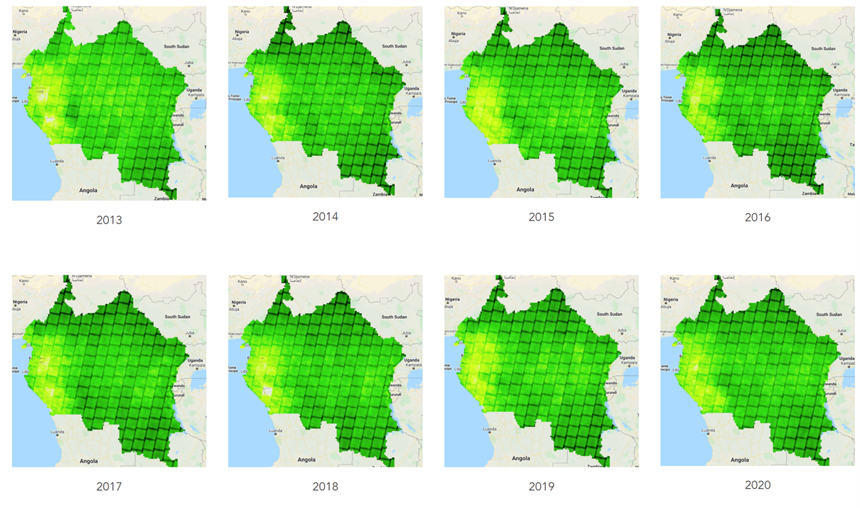
We evaluated the availability of Landsat 4, 5, 7 and 8 images for the creation of optical mosaics for the baseline year (2015). As you can see from the figure below, only certain sensors are available for certain time periods – from 2003 onwards the Landsat 7 sensor experienced a malfunction which results in data gaps in strips. This sensor should be only included when necessary (i.e. when not enough imagery is available). Luckily in SEPAL, the selection of sensors is automatic based on the selected date and only provides the available options.

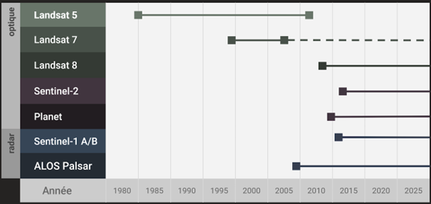
The coverage of Landsat over time is shown below (the western part of the study region along the coast; results in cloudy or data gaps in Cameroon, Equatorial Guinea and Gabon).

To create our optical mosaic, we will use the SEPAL Optical mosaic recipe (to learn more about the different available parameters and how to use the recipe, see Optical mosaics).

In this example, we will use a custom asset from GEE for the AOI parameter: projects/cafi_fao_congo/aoi/cafi_countries_buffer_simple. It includes an ISO column to select Congo Basin countries according to their three-digit code (for more information on AOI selection methods, see AOI selection).

In the DAT section, select the dates of interest.

For more recent years (after 2018), the sensor coverage is good, so you can safely select all images from a single year.

For less recent years (e.g. 2015) use the advanced option to add images from prior years from a targeted season (in this case the full year). This will help to fill gaps in cloudy areas.

For data sources, more is generally better. Select all Landsat options for a consistent mosaic. If you like, Sentinel-2 can be added for more data, but as the tiling system of the two sensors are different, you will be forced to use all available images (the option to select images will not be available).

If you have a lot of time to devote to your mosaic and you are working only with Landsat or Sentinel, you can manually select scenes to tailor your mosaic to your particular needs (USE ALL SCENES is the quickest, simplest approach, recommended for large areas).

For composite options, we recommend SR and BRDF; you can exclude pixels with low NDVI (particularly if you have a long time period) and select options presented in the following paragraph.

You can retrieve the mosaic as a Google asset at 30 m resolution. We select the original bands, as all other indices can be recalculated later: BLUE, GREEN, RED, NIR, SWIR1, SWIR2, and THERMAL.

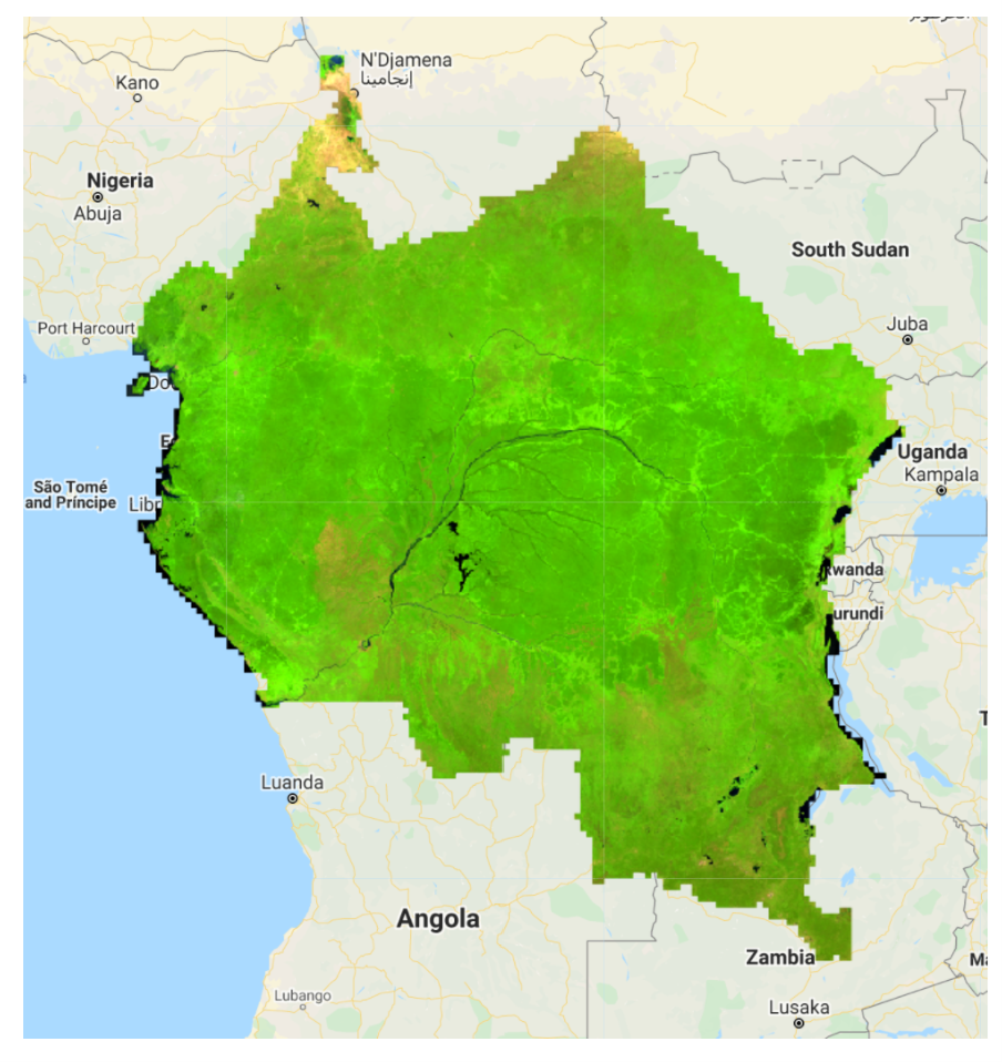
Once the export is finished, you can view the asset in GEE or SEPAL (see figure below of the 2015 mosaic of the Congo Basin using the above parameters).

ALOS PALSAR mosaics

Radar imagery has the added benefit of being cloud-free by design, as active sensors are not influenced by clouds.

The Advanced Land Observation Satellite - Phased Array type L-band Synthetic Aperture Radar (ALOS PALSAR) is an L-band radar that gives good results for monitoring forest ecosystems. Data is provided by the Kyoto & Carbon Initiative from the Japanese Space Agency (JAXA) for the year 2015 onward. SEPAL provides an application to select; process and download them to your SEPAL workspace or GEE account.

For more information about the parameters, please see ALOS K&C mosaics.

Sentinel-1 mosaics

You can use the Sentinel-1 recipe to create a mosaic from European Space Agency (ESA) Copernicus radar data.

The AOI selection is the same as for the optical mosaic.

For the dates, you can enter a year, a date range or a single date. When you add a year or date range, SEPAL will provide a “time-scan” composite that includes bands which are statistical metrics of the range of data, including phase and amplitude, which assess the phenology and variations within the time period.

For the best results in the Congo Basin, the following parameters are proposed:

• Both Ascending and Descending orbits will ensure complete coverage of the AOI.

• The Terrain correction will mask any errors due to topography or terrain “shadows”.

• We don’t need to apply a speckle filter.

• Moderate outlier removal will provide the most consistent results.

Select which bands to export in the Retrieve window. You may select all of them depending on the space available in your GEE repository or SEPAL workspace.

Resolution can also be selected accordingly – you can choose 30 to be at the same scale as the optical mosaic, which will be classified in the next step.

Time-series analysis

Attention

This part of the documentation is still under construction.

Sample stratification

Attention

This part of the documentation is still under construction.

Identification of direct drivers

Direct drivers of forest change and disturbance are multiple, overlapping and interacting, as deforestation and degradation cannot be reduced to one single cause. Therefore, the assessment specifically analyses the various combinations of overlapping drivers, providing context and richness.

The scope of the assessment is to identify the multiple direct drivers of deforestation and degradation in areas of forest disturbance. As a result, this assessment can:

• determine where direct drivers are present and overlap in areas of forest disturbance;

• assess the relative contribution of direct drivers in the region/country;

• determine direct drivers relative to forest type and fragmentation class; and

• determine the relative weight of direct drivers over time (in relation to the date of detected disturbance).

The analysis performed is a drivers assessment – not a land cover change analysis. A land cover change map or fate of land post–disturbance, where forest loss is measured in terms of area of land cover or use, is produced through different approaches than employed here. Furthermore, a land cover or pixel-level analysis simply does not consider driver context. Finally, land cover maps do not address the drivers of forest degradation (where disturbance occurs, but the land cover is still forest) which is a crucial element of this study.

The project’s technical committee agreed upon nine unique direct drivers and their characteristics to be used in the context of the project, as well as its piloting in Central Africa. The definitions were based on what is potentially visible and recognizable in high-resolution satellite imagery mosaics from Planet that are available over the entire study period (2015–2020). Each driver and its definition and characteristics are described in Direct driver definitions.

In order to identify direct drivers, a survey form is used in the CEO web platform to enable visual interpretation and identification of the presence or absence of forest, the land cover type in 2015, the type of change (deforestation or degradation) and the year of change (2015–2022), along with one or more observed direct drivers within a 2 km wide square plot around the sample point.

References

Curtis, P.G., Slay, C.M., Harris, N.L., Tyukavina, A. & Hansen, M.C. 2018. Classifying drivers of global forest loss. Science, 361(6407): 1108–1111. https://doi.org/10.1126/science.aau3445

FAO (Food and Agriculture Organization of the United Nations). 2022. FRA 2020 Remote Sensing Survey. FAO. https://doi.org/10.4060/cb9970en

Ferrer-velasco. 2020.

Gibbs, H.K., Ruesch, A.S., Achard, F., Clayton, M.K., Holmgren, P., Ramankutty, N. & Foley, J.A. 2010. Tropical forests were the primary sources of new agricultural land in the 1980s and 1990s. Proceedings of the National Academy of Sciences, 107(38): 16732–16737. https://doi.org/10.1073/pnas.0910275107

Hosonuma, N., Herold, M., De Sy, V., De Fries, R.S., Brockhaus, M., Verchot, L., Angelsen, A. & Romijn, E. 2012. An assessment of deforestation and forest degradation drivers in developing countries. Environmental Research Letters, 7(4): 044009. https://doi.org/10.1088/1748-9326/7/4/044009

Kissinger, G., M. Herold and De Sy, V. 2012. Drivers of Deforestation and Forest Degradation: A Synthesis Report for REDD+ Policymakers. Vancouver, Canada, Lexeme Consulting.

Molinario, G., Hansen, M., Potapov, P., Tyukavina, A. & Stehman, S. 2020. Contextualizing Landscape-Scale Forest Cover Loss in the Democratic Republic of Congo (DRC) between 2000 and 2015. Land, 9(1): 23. https://doi.org/10.3390/land9010023

Sandker, M., Finegold, Y., D’Annunzio, R. & Lindquist, E. 2017. Global deforestation patterns: comparing recent and past forest loss processes through a spatially explicit analysis. International Forestry Review, 19(3): 350–368. https://doi.org/10.1505/146554817821865081