

Séries temporelles#
Create and retrieve SITS to study patterns and key changes in landscape evolution over time
Présentation#
Une Satellite Image Time Series (SITS) est un ensemble d’images satellites prises de la même scène à différents moments. Un SITS utilise différentes sources satellites pour obtenir une plus grande série de données avec un bref intervalle de temps entre deux images. Dans ce cas, il est fondamental de respecter la résolution spatiale et les contraintes d’enregistrement.
Satellite observations offer opportunities for understanding how the Earth is changing, determining the causes of these changes and predicting future changes. Remotely sensed data, combined with information from ecosystem models, offer an opportunity for predicting and understanding the behaviour of Earth’s ecosystems. Sensors with high spatial and temporal resolutions make the observation of precise spatio-temporal structures in dynamic scenes more accessible. Temporal components integrated with spectral and spatial dimensions allow the identification of complex patterns concerning applications connected with environmental monitoring and analysis of land cover dynamics.
La détection des changements ne peut fournir qu’un scénario « avant et après » ; une analyse de séries temporelles offre l’occasion d’étudier les modèles et les changements clés dans l’évolution du paysage au fil du temps.
This SEPAL recipe allows users to create and retrieve SITS based on Landsat and Copernicus programmes” imagery using the Google Earth Engine (GEE) datacube.
Attention
Vous ne serez pas en mesure de télécharger des images si votre compte SEPAL et GEE n’est pas connecté. Pour en savoir plus, allez à Connecter SEPAL à GEE.
Commencer#
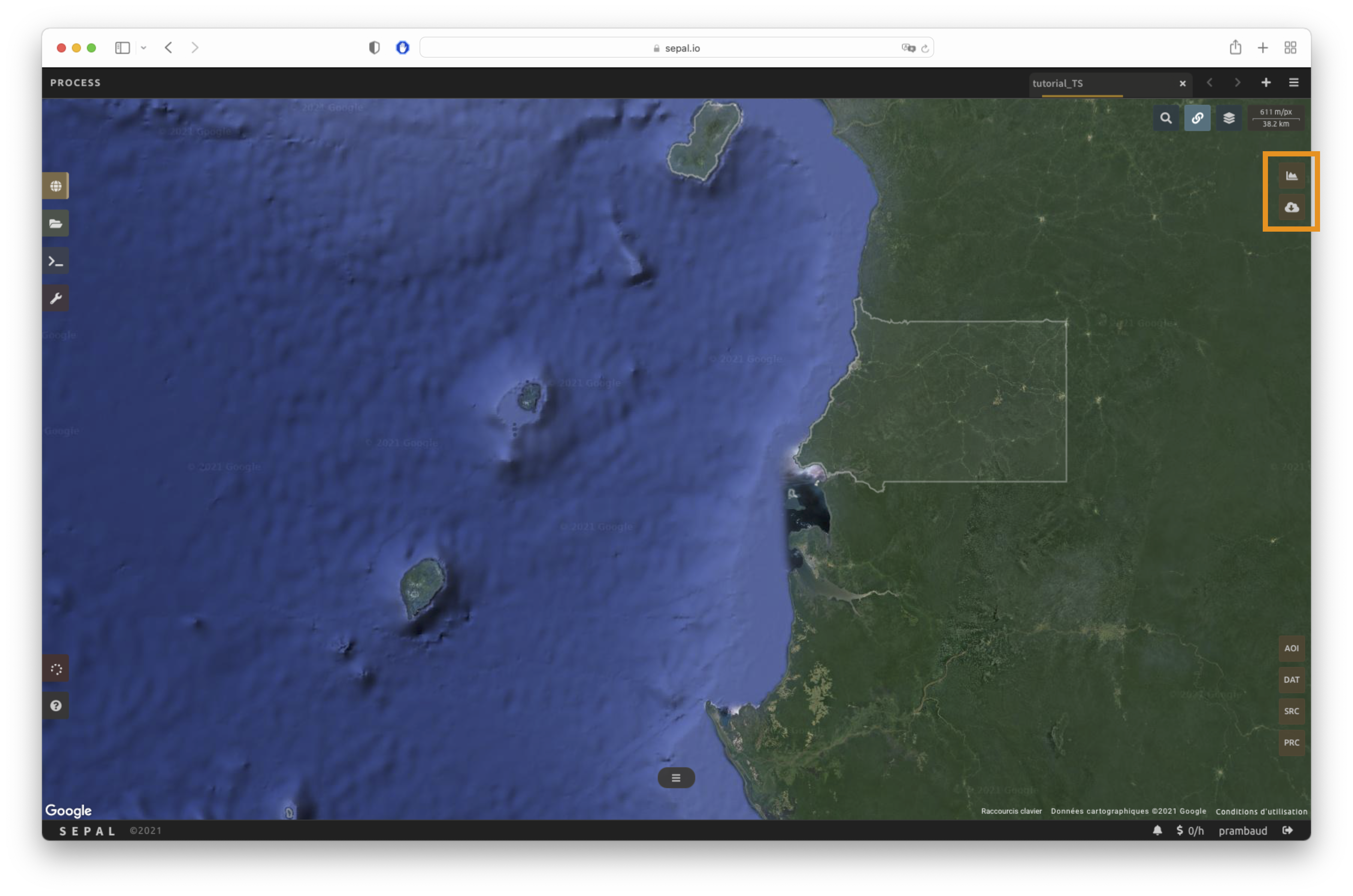
Once the Time series recipe is selected, SEPAL will open the recipe process in a new tab (see 1 in the following figure). The base map will change to Google high-resolution imagery and the Area of interest (AOI) selection window will appear in the lower right (2).
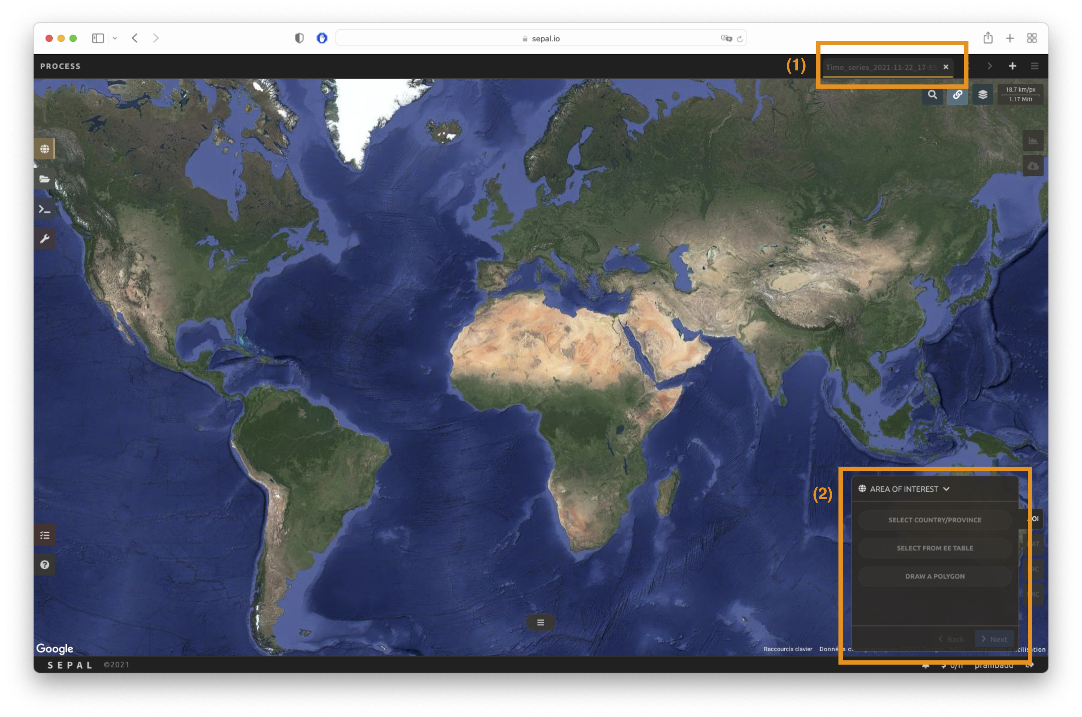
La première étape est de changer le nom de la recette. Ce nom sera utilisé pour identifier vos fichiers et recettes dans les dossiers SEPAL. Utilisez la convention la mieux adaptée à vos besoins. Double-cliquez simplement sur l’onglet et entrez un nouveau nom. Il sera par défaut à Time_series_<start_date>_<end_date>_<band name>.

Note
L’équipe SEPAL recommande d’utiliser la convention de nommage suivante : <aoi name>_<start-<end>_<measure>_<sensors> (ex : sgp_2012-2018_ndfi_l78).
Paramètres#
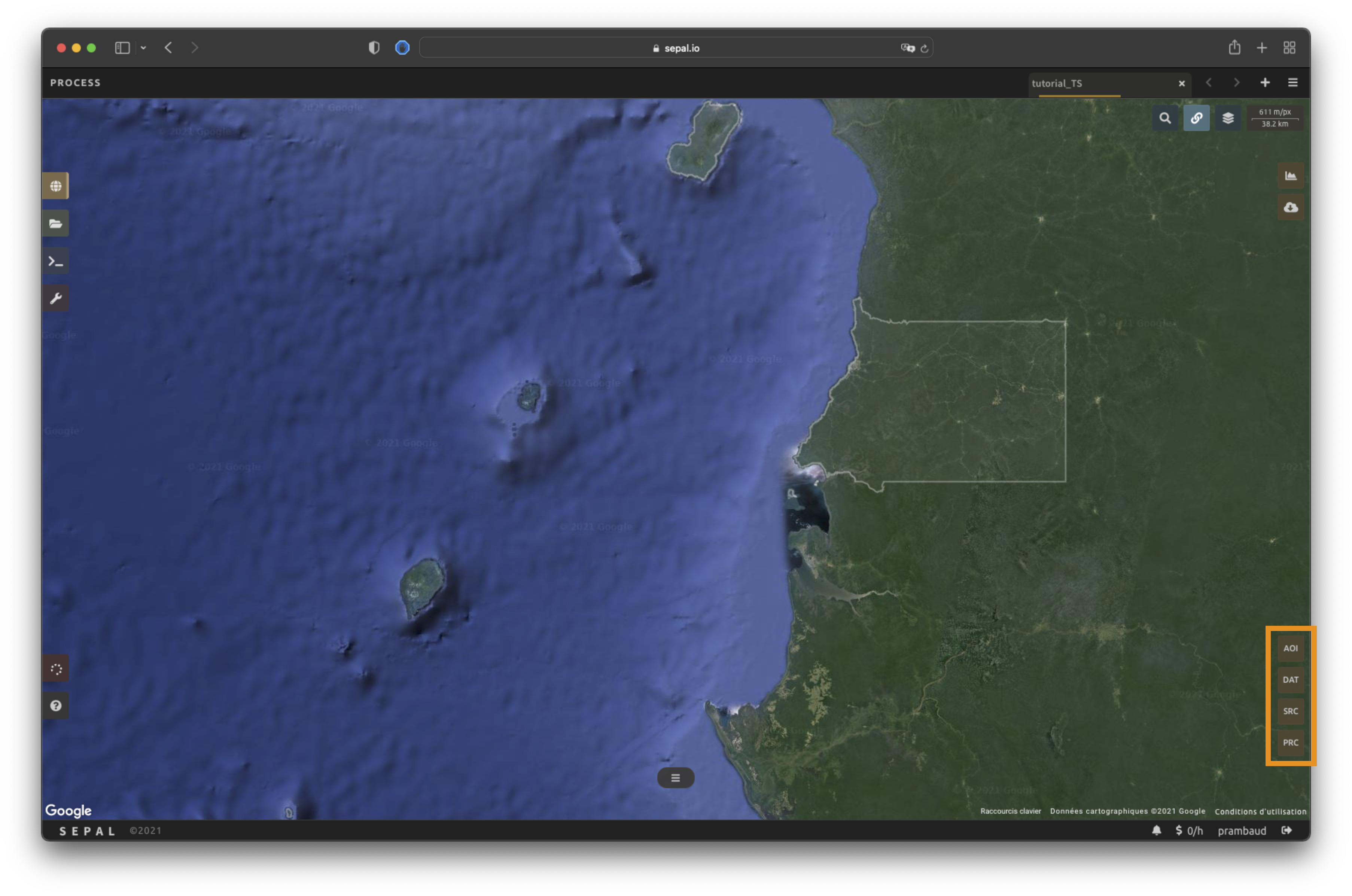
In the lower-right corner, four tabs are available, allowing you to customize the time series to your needs:
AOI: area of interest (AOI)
DAT: dates of the time series
SRC: source datasets of the time series
PRC: pre-processing parameters
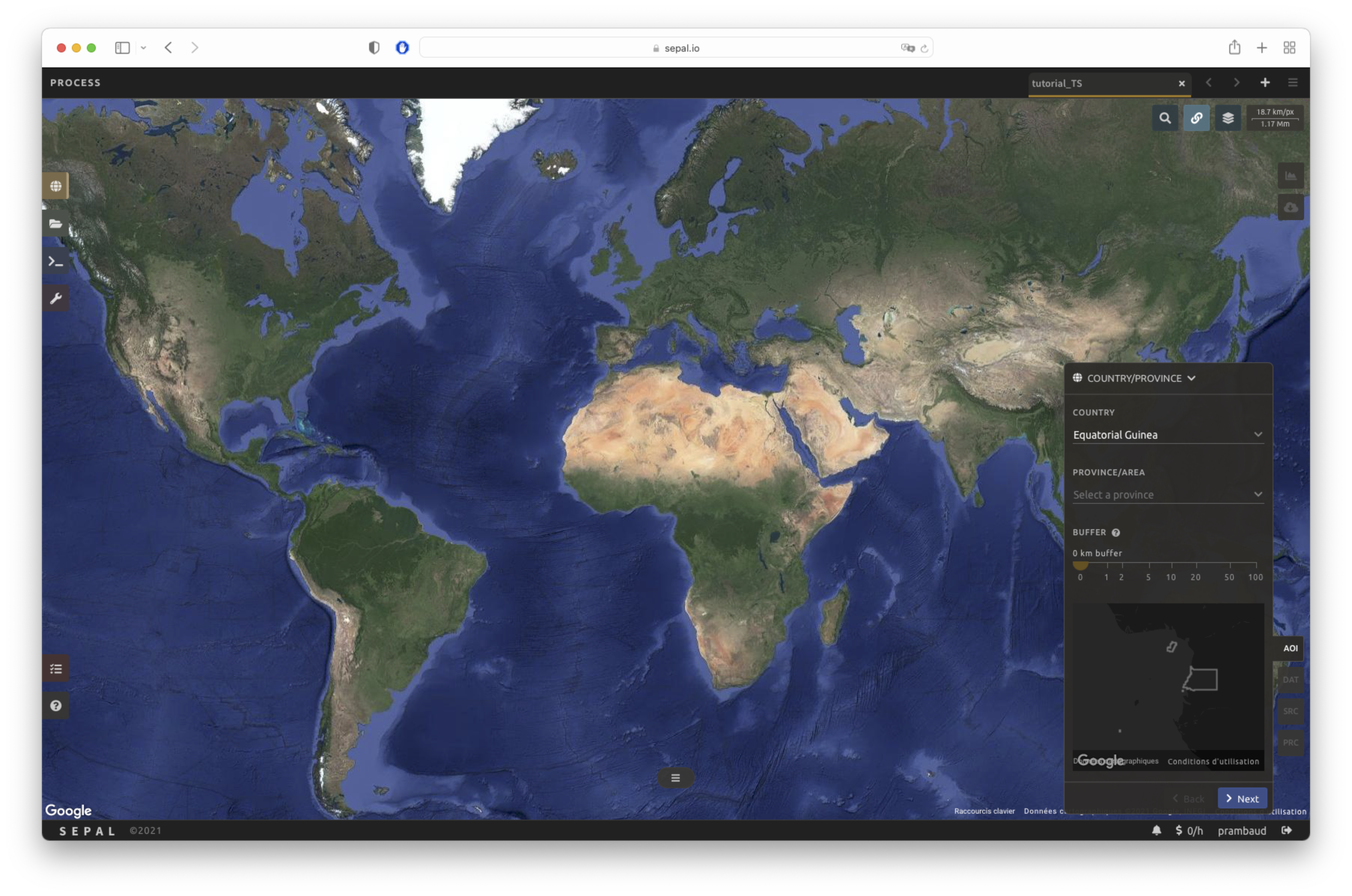
Sélection de l’AOI#
Les données exportées par la recette seront limitées aux limites de l’AOI. Il y a plusieurs façons de sélectionner l’AOI dans SEPAL:
Limites administratives
Tables EE
Polygones personnalisés
Pour plus d’informations, allez à Sélection de l’AOI.
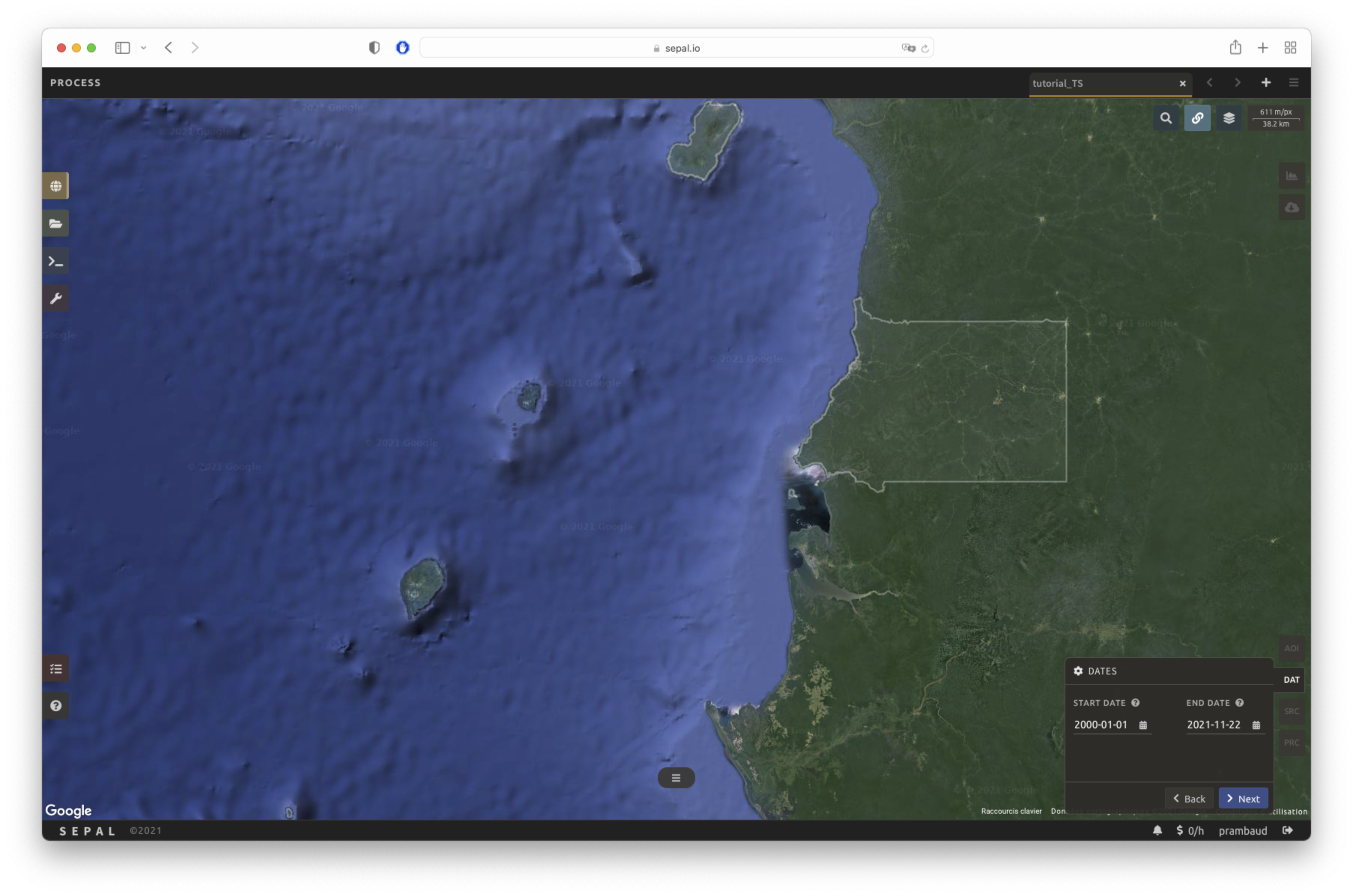
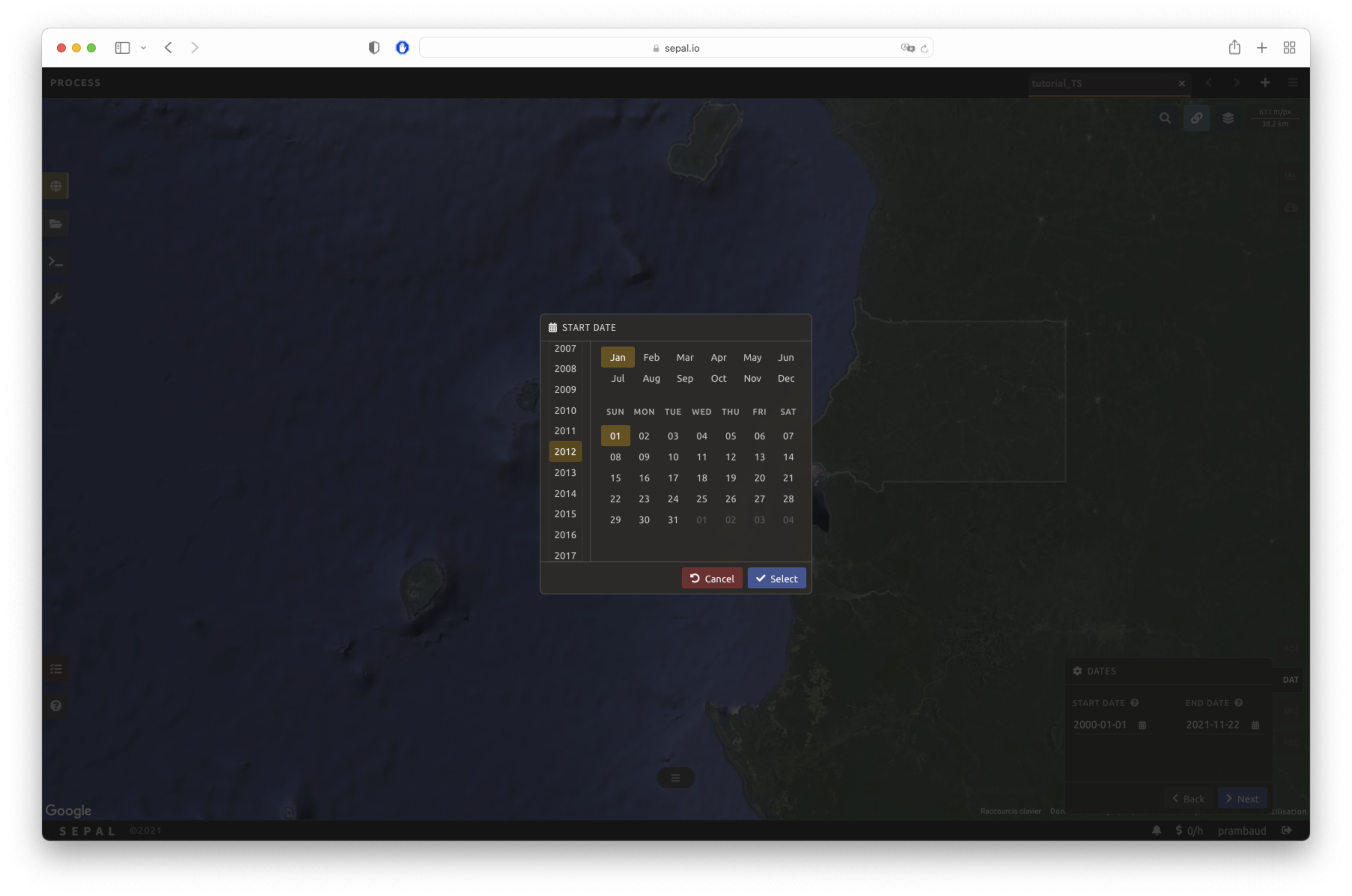
Dates#
Dans l’onglet DAT, il vous sera demandé de sélectionner la date de début et la date de fin de la série horaire. Sélectionnez le champ de texte Date pour ouvrir une fenêtre popup. Choisissez le bouton Select pour choisir une date. Lorsque les deux dates ont été choisies, sélectionnez le bouton Appliquer.
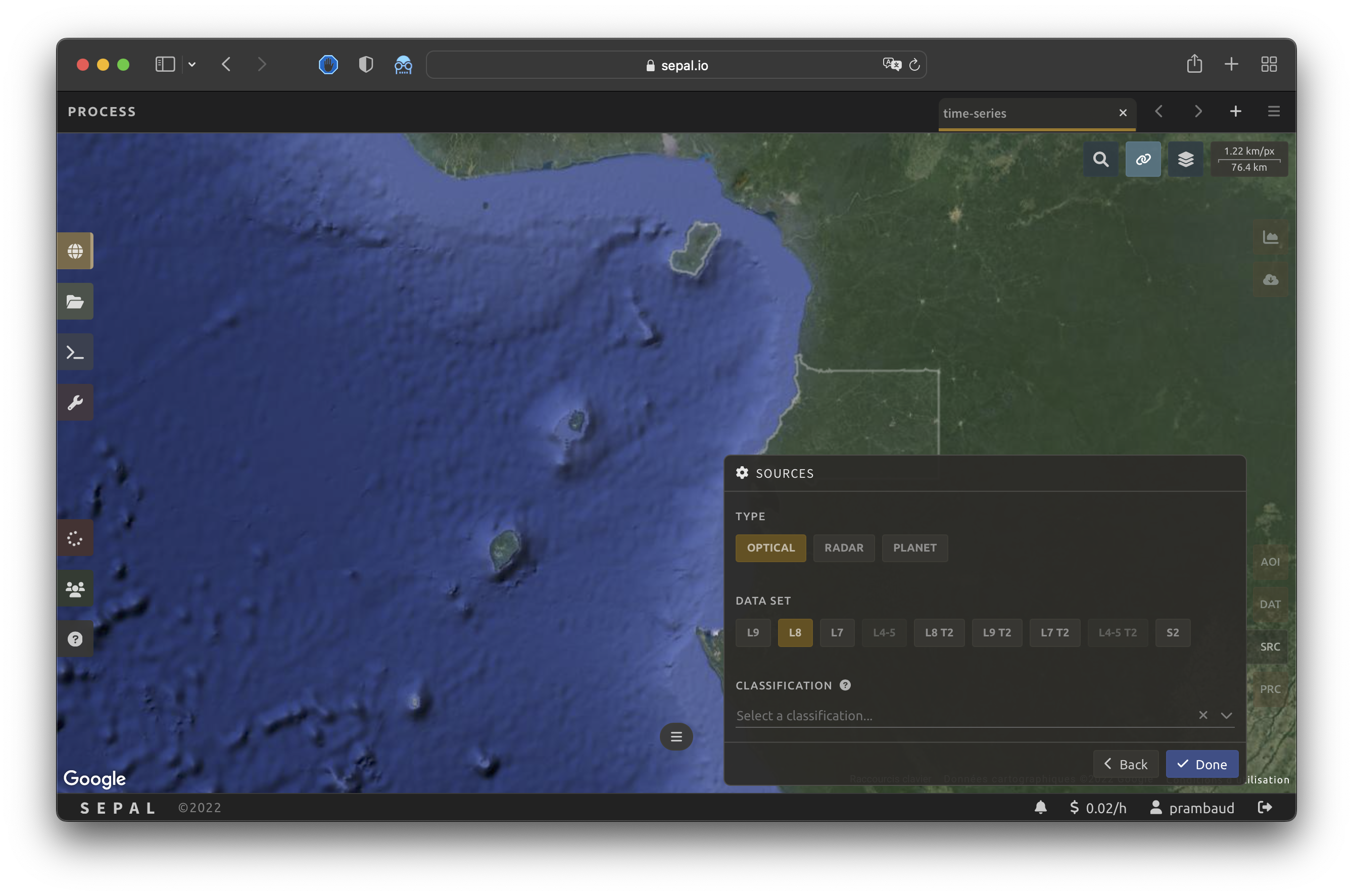
Sources#
Comme mentionné dans l’introduction, un SITS utilise différentes sources satellites pour obtenir une plus grande série de données avec un intervalle de temps plus court entre les images. Pour atteindre cet objectif, SEPAL vous permet de sélectionner des données à partir de plusieurs points d’entrée. Vous pouvez sélectionner plusieurs sources dans les jeux de données Radar, Optical ou Planet.
Lorsque toutes les données ont été sélectionnées, sélectionnez Appliquer.
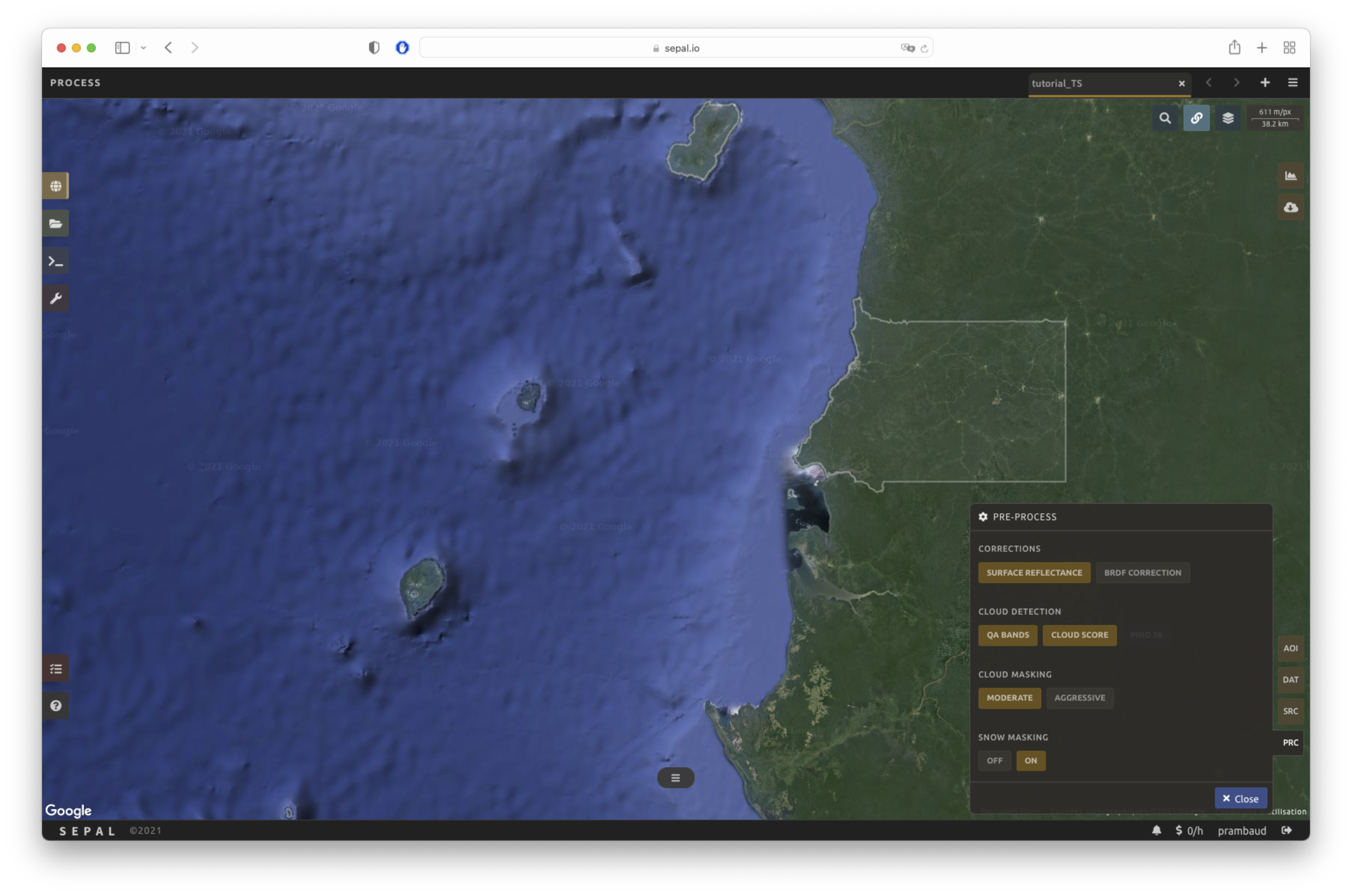
Prétraitement#
Note
Cette section est optionnelle car ces paramètres sont définis par défaut.
Correction:
AucunDétection de nuage: Bandes QA, Score Cloud
Masquage de nuage: modéré
Masquage des neiges: activé
Multiple pre-processing parameters can be set to improve the quality of the provided images. SEPAL has gathered four of them in the form of these interactive buttons. If you think others should be added, tell us in the issue tracker.
Correction
Réflexion de surface: Utiliser des scènes avec la réflexion de surface corrigée pour les effets atmosphériques.
:guilabel:`Correction BRDF`Corriger les effets de réflectance bidirectionnelle de distribution (BRDF).
Détection des nuages
QA bands: Use previously created quality assessment (QA) bands from datasets.
Score Cloud: Utilisez un algorithme avec un score de couverture nuageuse.
Masquage des nuages
Modéré: Ne comptez que sur les bandes QA des images sources pour le masquage des nuages.
Aggressive: Rely on image source QA bands and a cloud-scoring algorithm for cloud masking (this will probably « mask » some built-up areas and other bright features).
Snow masking
On: Mask snow (this tends to leave some pixels with shadowy snow).
Off: Don’t mask snow (some clouds might get misclassified as snow, and because of this, disabling snow masking might lead to cloud artefacts).
Bandes disponibles#
Note
The wavelength of each band is dependent on the satellite used.
The time series will use a single observation for each pixel. This observation can be one of the available bands in SEPAL. To discover the full list of available bands, see Optical Satellite bands, transformations, and indices and ../feature/radar_bands.
Analyse#
Once all parameters are set, you can generate data from the recipe. Some can be directly generated on the fly from the interface; the rest require retrieving the data from SEPAL folders.
Les icônes d’analyse se trouvent dans le coin supérieur droit de l’interface SEPAL :
: Tracer les données.
: Retrieve data.
Astuce
The Download icon is only enabled when the data parameters are complete. If the button is disabled, check your parameters, as some might be missing.
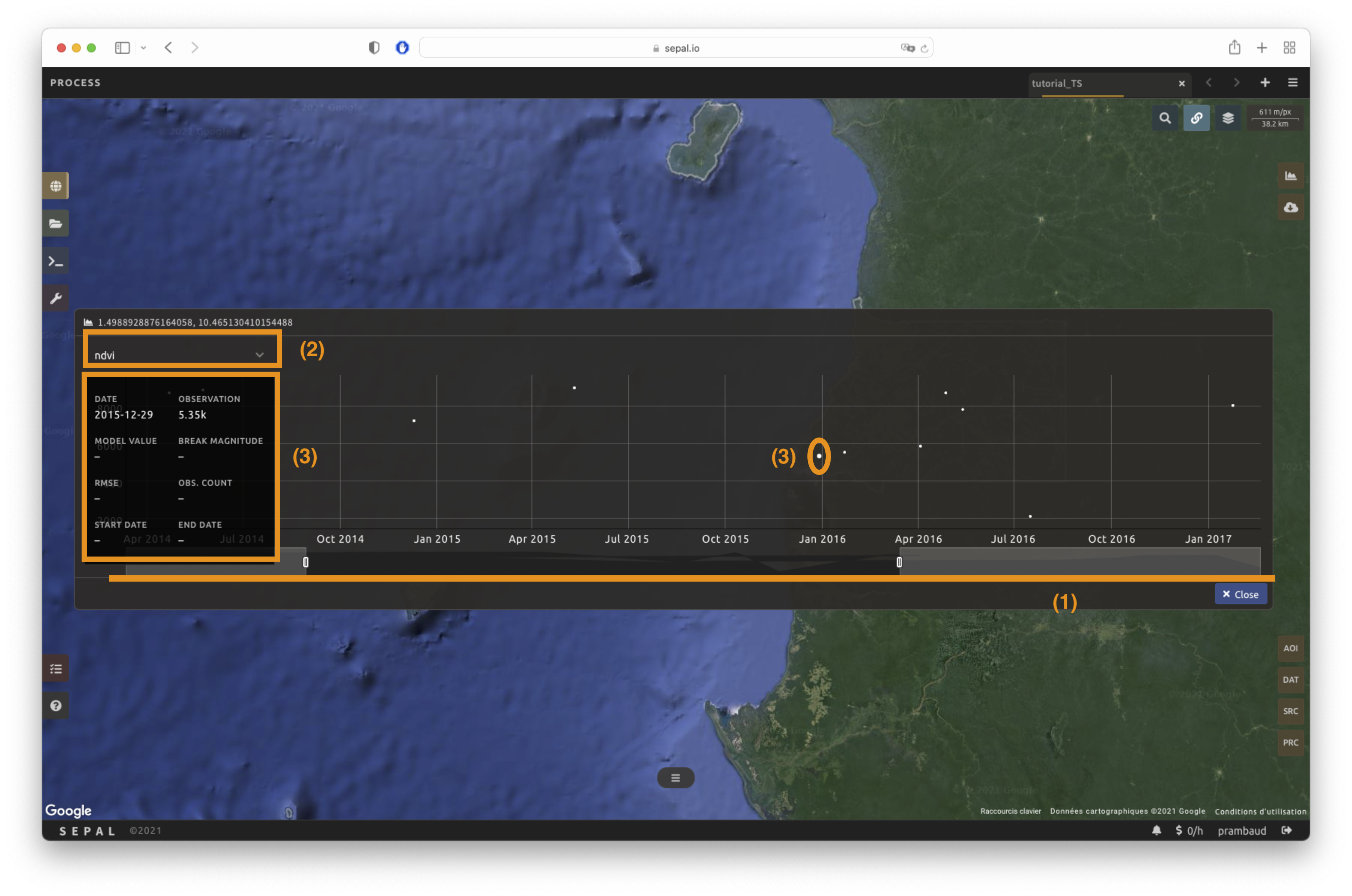
Plot#
Select to start the plotting tool. Move the pointer to the main map; the pointer will be transformed into a . Click anywhere in the AOI to plot data for this specific location in the following pop-up window.
The plotting area is dynamic and can be customized by the user.
Using the slider (1), the temporal width displayed can be changed. It cannot exceed the start and/or end date of the time series.
You can also select the observation feature by selecting one of the available measures in the dropdown selector in the upper-left corner (2). The available bands are the same as those described previously.
On the main graph, each point represents one valid observation (based on the pre-processing filters). Hover over the point to let the tooltip describe the value and date of the observation (3).
Astuce
The coordinates of the point are displayed at the top of the chart window.
Attention
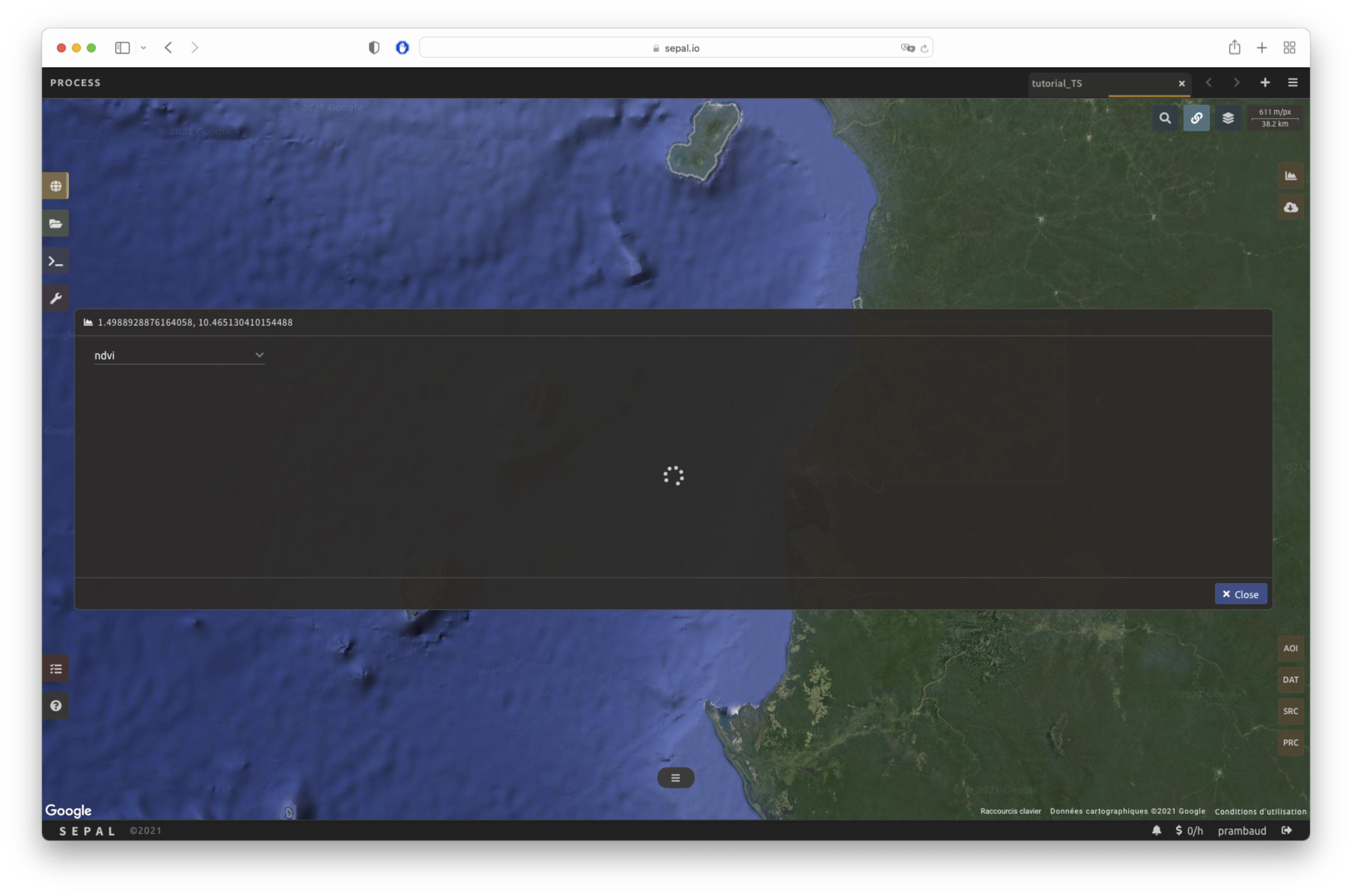
Since the plot feature is retrieving information from GEE on the fly and presenting it in an interactive window, this operation can take time, depending on the number of available observations and the complexity of the selected pre-processing parameters. If a spinning wheel appears in the pop-up window, you may have to wait up to two minutes to see the data displayed.
Exporter#
In order for the data generated by the recipe to be used in other workflows, it needs to be retrieved from GEE and uploaded to SEPAL.
Important
You cannot export a recipe as an asset or a .tiff file without a small computation quota. If you are a new user, see Gérer vos ressources.
Paramètres#
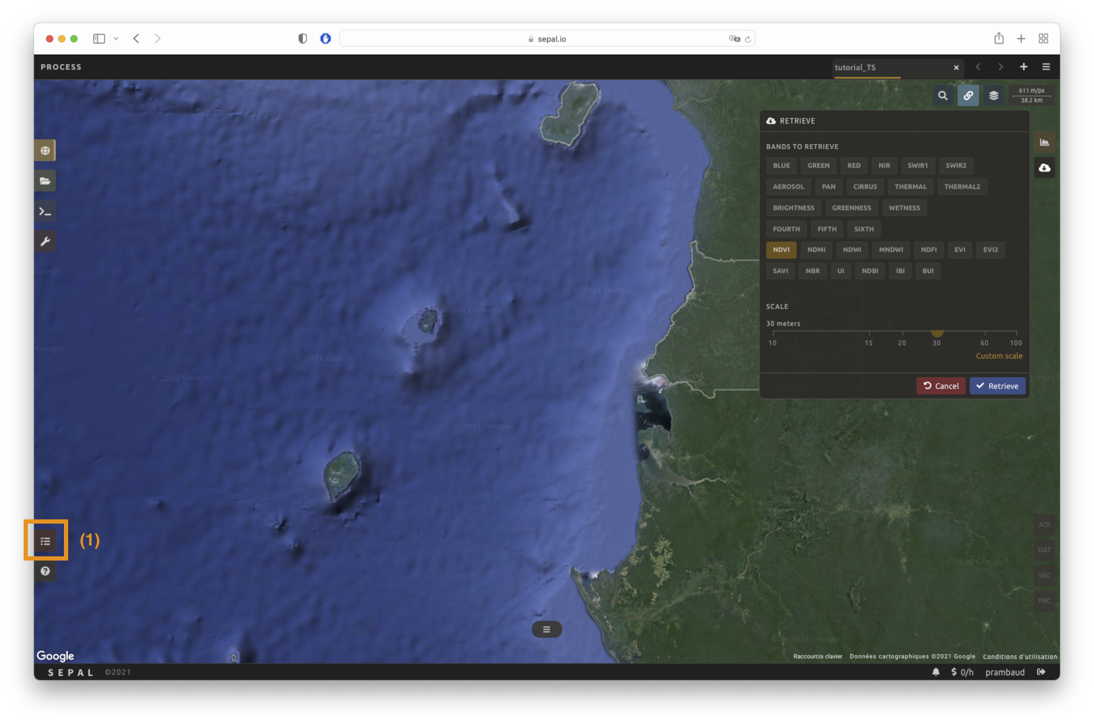
Select to open the Download parameters window. You will be able to select the measure to use on each observation of the time series. This measure can be selected in the list of available bands presented above in a previous section.
Note
There is no fixed rule to the measure selection. Each index is more adapted to a set of analyses in a defined biome. The knowledge of the study area, the evolution expected and the careful selection of an adapted measure will improve the quality of downstream analysis.
You can set a custom scale for exportation by changing the value of the slider in metres (m). Keep in mind that Sentinel data native resolution is 10 m and Landsat is 30 m.
When all the data is selected, select the apply button. Notice that the task tab in the lower-left corner of the screen (1) will change from to , meaning that the tasks are loading.
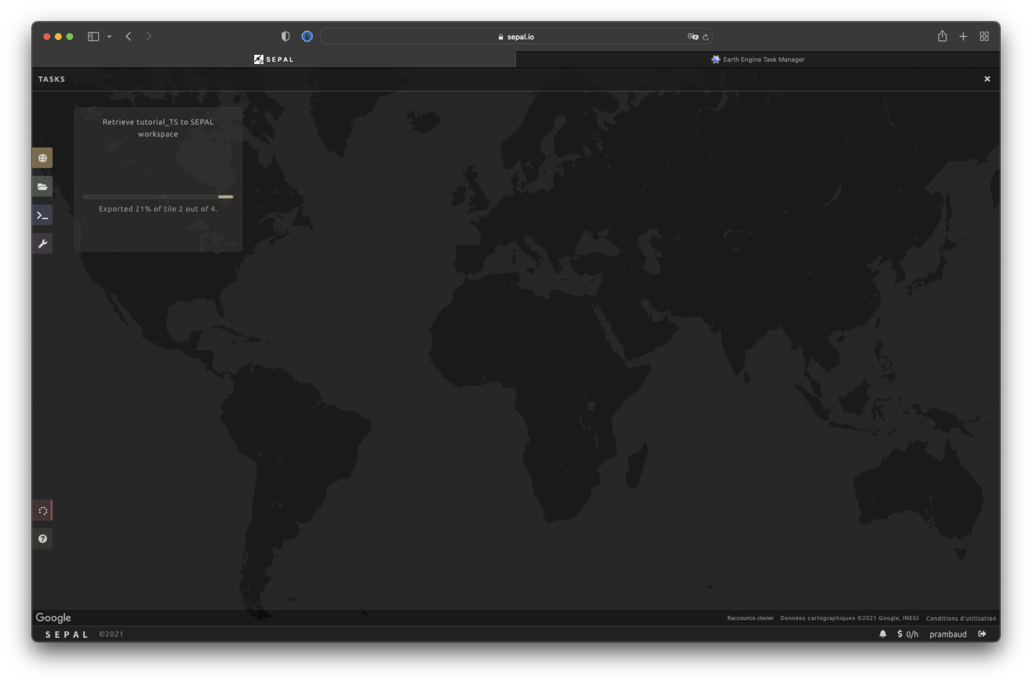
État d’exportation#
By selecting the Tasks tab (lower-left corner using the or buttons, depending on the loading status), you will see the list of different tasks loading. The interface will provide you with information about the task progress and display an error if the exportation has failed. If you are unsatisfied with the way we present information, the task can also be monitored using the GEE task manager.
Astuce
This operation is running between GEE and SEPAL servers in the background, so you can close the SEPAL page without ending the process.
When the task is finished, the frame will be displayed in green, as shown in the second image below.

Access#
Once the download process is done, you can access the data in your SEPAL folders in Downloads, using the following format:
.
└── downloads
    └── <TS name>
        ├── <tile number>
        │   ├── chunk-<start date>_<end date>
        │   │   ├── <TS name>_<tile number>_<start_date>_<end date>-<gee tiling id>.tif
        │   │   ├── ...
        │   │   └── <TS name>_<tile number>_<start_date>_<end date>-<gee tiling id>.tif
        │   ├── ...
        │   ├── chunk-<start date>_<end date>
        │   ├── tile-<gee tiling id>
        │   │   └── stack.vrt
        │   ├── ...
        │   ├── tile-<gee tiling id>
        │   ├── dates.csv
        │   └── stack.vrt
        ├── ...
        └── <tile number>
Important
Understanding how images are stored in a time series is only required if you want to manually use them. The SEPAL applications are bound to this tiling system and can digest this information for you.
The data are stored in a folder using the name of the time series as it was labeled in the first section of this document. The SEPAL team was forced to use this folder structure as GEE is unable to export an ee.ImageCollection. As the data is spatially too big to be exported at once, they are divided into smaller pieces and reassembled in a stack.vrt file.
The AOI provided by the user will be divided into multiple SEPAL tiles. The AOI is a ee.FeatureCollection; each feature is downloaded in a different tile. If the tile is bigger than 2° x 2° (EPSG:4326), then the feature is divided again until all of the tiles are smaller than the maximum 2° size. The tiles are identified by their <tile_number>.
To limit the size of the downloaded images, in each SEPAL tile, the time period is divided into Chunks of 3 months. They are identified by their <chunk-<start>_<end>. Chunks are image folders. As a SEPAL tile is still bigger than what GEE can download at once, the images are divided into GEE tiles. This tiling process uses its own identification system (000000xxxx-000000xxxx). Consequently, Chunks contain tile raster images. Each one of these images is composed of one band per observation date, with the value of the measure for each pixel. The bands are named with the date.
To gather all these rasters together, a first aggregation on time is performed. One stack.vrt is created per GEE tile, meaning that each stack.vrt file contains all the *<gee tiling id>.tif contained in each Chunk, reconstituting the full time period on the smallest spatial unit: the GEE tile. Each file is stored in a folder called tile-<gee tiling id>.
Finally, information is gathered spatially at the SEPAL tile level in the main stack.vrt file.
The last file, date.csv, gathers all the observation dates in chronological order.
Note
The dates contained in date.csv can differ from one SEPAL tile to another, due to data availability and pre-processing filters.
Astuce
Le dossier complet avec une arborescence cohérente est nécessaire pour lire le fichier .vrt
Voici un exemple d’un vrai dossier de Serie Temporelle :
.
└── downloads
    └── tutorial_TS
        ├── 1
        │   ├── chunk-2012-01-01_2012-04-01
        │   │   ├── tutorial_TS_1_2012-01-01_2012-04-01-0000000000-0000000000.tif
        │   │   ├── ...
        │   │   └── tutorial_TS_1_2012-01-01_2012-04-01-0000002560-0000001024.tif
        │   ├── ...
        │   ├── chunk-2018-10-01_2018-12-31
        │   ├── tile-0000000000-0000000000
        │   │   └── stack.vrt
        │   ├── ...
        │   ├── tile-0000002560-0000001024
        │   ├── dates.csv
        │   └── stack.vrt
        ├── ...
        └── 3
Important
Now that you have downloaded the TS to your SEPAL account, it can be downloaded to your computer using FileZilla or used in one of our Time-series analysis modules.