

Mosaïques optiques#
Combine images to create single raster datasets with optical mosaics
Aperçu#
A mosaic is a combination or fusion of two or more images. In SEPAL, you can create a single raster dataset from several raster datasets by mosaicing them together. This can be achieved on both contiguous rasters (see first image below) and overlapping images (see second image below).
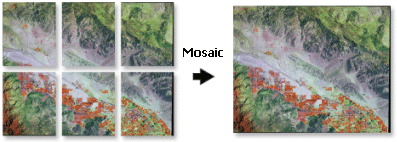
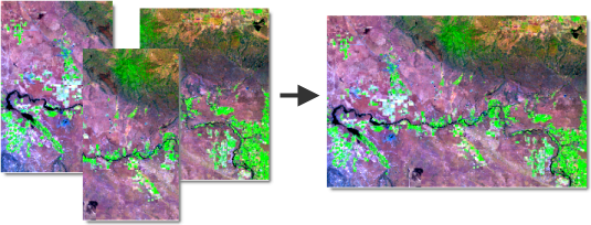
Ces zones de superposition peuvent être gérées de différentes manières. Par exemple, vous pouvez choisir de:
ne conserve que les données matricielles du premier ou dernier jeu de données ;
combiner les valeurs des cellules de superposition à l’aide d’un algorithme de pondération ;
moyenner les valeurs des cellules de superposition ; ou
prend la valeur maximale ou minimale.
En outre, certaines corrections peuvent être apportées à l’image pour tenir compte des nuages, de la neige et d’autres facteurs; ces opérations sont complexes et répétitives.
SEPAL vous offre un moyen interactif et intuitif de créer des mosaïques dans n’importe quel zone d’intérêt (AOI).
Note
Vous ne pourrez pas récupérer les images si vos comptes SEPAL et Google Earth Engine (GEE) ne sont pas connectés. Pour plus d’informations, allez dans Use GEE with SEPAL.
Début#
Once the mosaic recipe is selected, SEPAL will display the recipe process in a new tab (see 1 in the image below) and the AOI selection window will appear in the lower right (2).
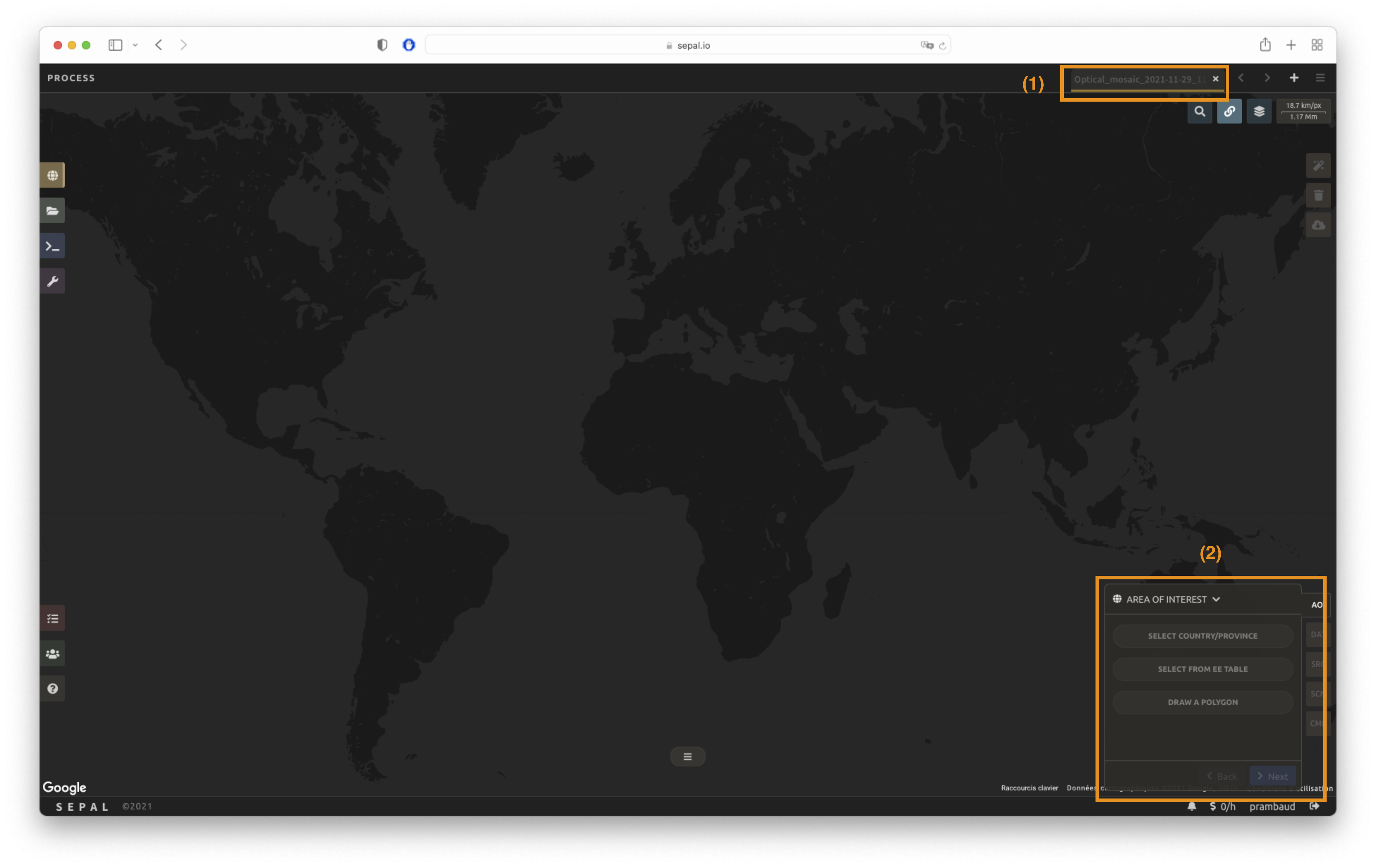
The first step is to change the name of the recipe. This name will be used to identify your files and recipes in SEPAL folders. Use the best-suited convention for your needs. Simply double-click the tab and write a new name. It defaults to Optical_mosaic_<start_date>_<end_date>_<band name>.


Note
L’équipe SEPAL recommande d’utiliser la convention suivante : <aoi name>_<dates>_<measure>.
Paramètres#
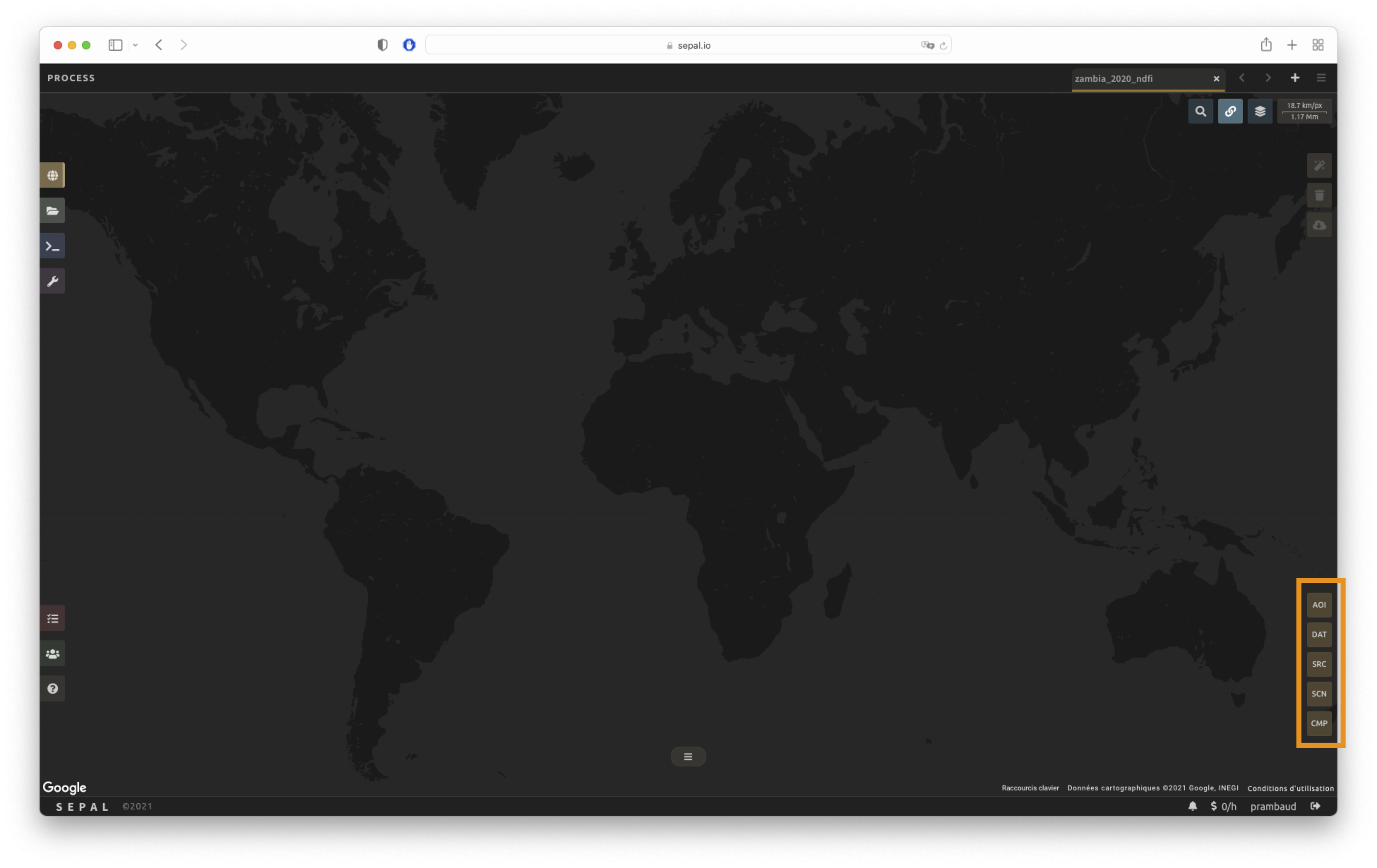
In the lower-right corner, five tabs are available, which allow you to customize the mosaic creation to your needs:
AOI: zone d’intérêt
DAT: date cible d’intérêt pour la mosaïque/composite
SRC: jeu de données source de la mosaïque/composite
SCN: paramètres de sélection de scène
CMP: paramètres de composition
Sélection de l’AOI#
Les données exportées par la recette seront générées à partir des limites de l’AOI. Il y a plusieurs façons de sélectionner l’AOI dans SEPAL:
Limites administratives
Tables EE
Polygones personnalisés
Ils sont décrits dans notre documentation. Pour plus d’informations, lisez Sélection de l’AOI.

Date#
Mosaïque annuelle#
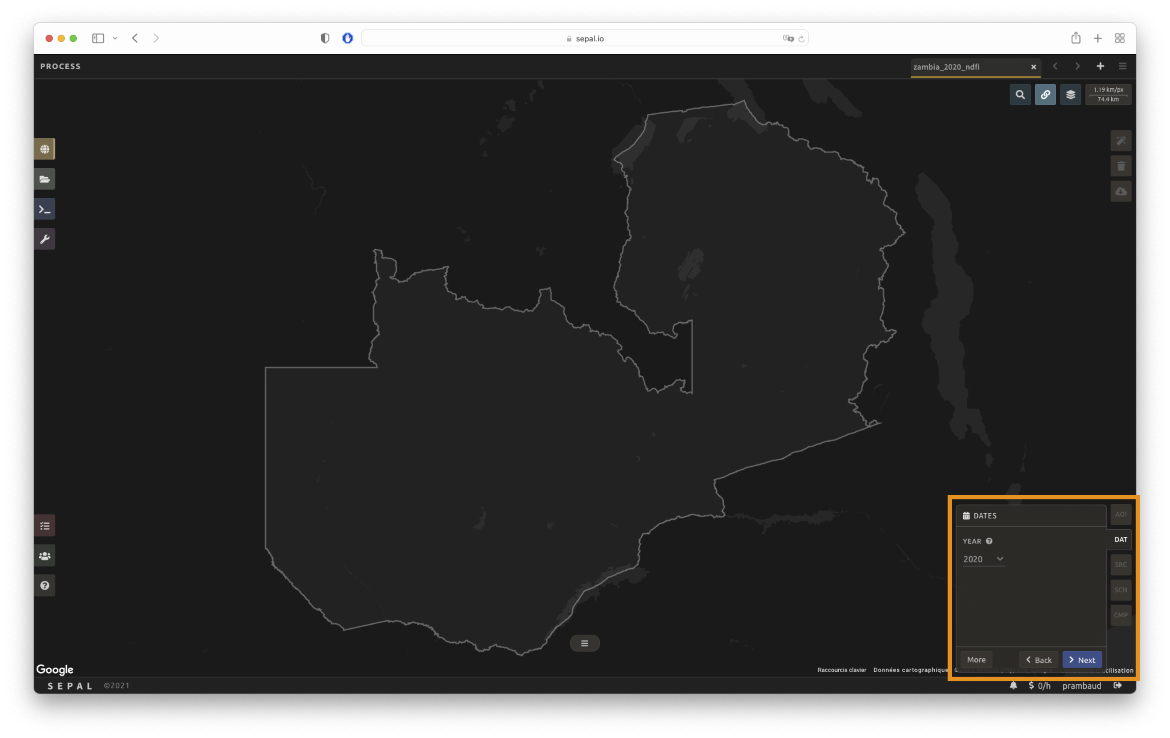
In the DAT tab, select a year which pixels in the mosaic should come from. Then select the Apply button.
Mosaïque saisonnière#
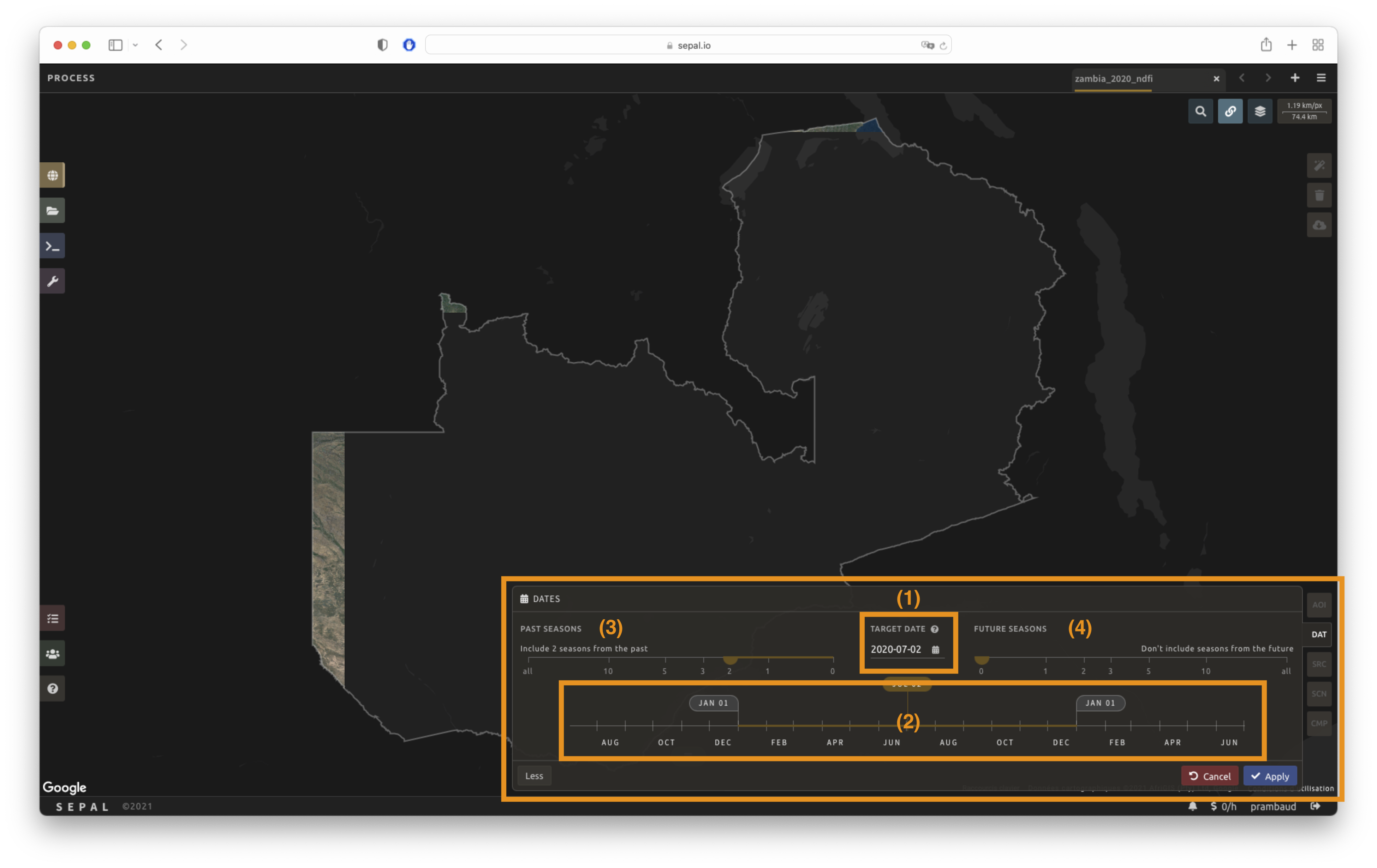
Sélectionnez Plus dans le panneau DAT pour étendre l’outil de sélection de date. Plutôt que de choisir une année, vous pouvez choisir une saison d’intérêt.
Select the (1) to open the Date selection pop-up window. The selected date will be the target of the mosaic (i.e. the date from which pixels in the mosaic should ideally come from).
Using the main slider (2), define a season around the target date by identifying a start date and end date. SEPAL will then retrieve the mosaic images between those dates.
The number of images in a single season of one year may not be enough to produce a correct mosaic. SEPAL provides two secondary sliders to increase the pool of images to create the mosaic. Both count the number of seasons SEPAL can retrieve in the past (Past season - [3]) and in the future (Future season - [4]).
When the selection is done, select the Apply button.
Sources#
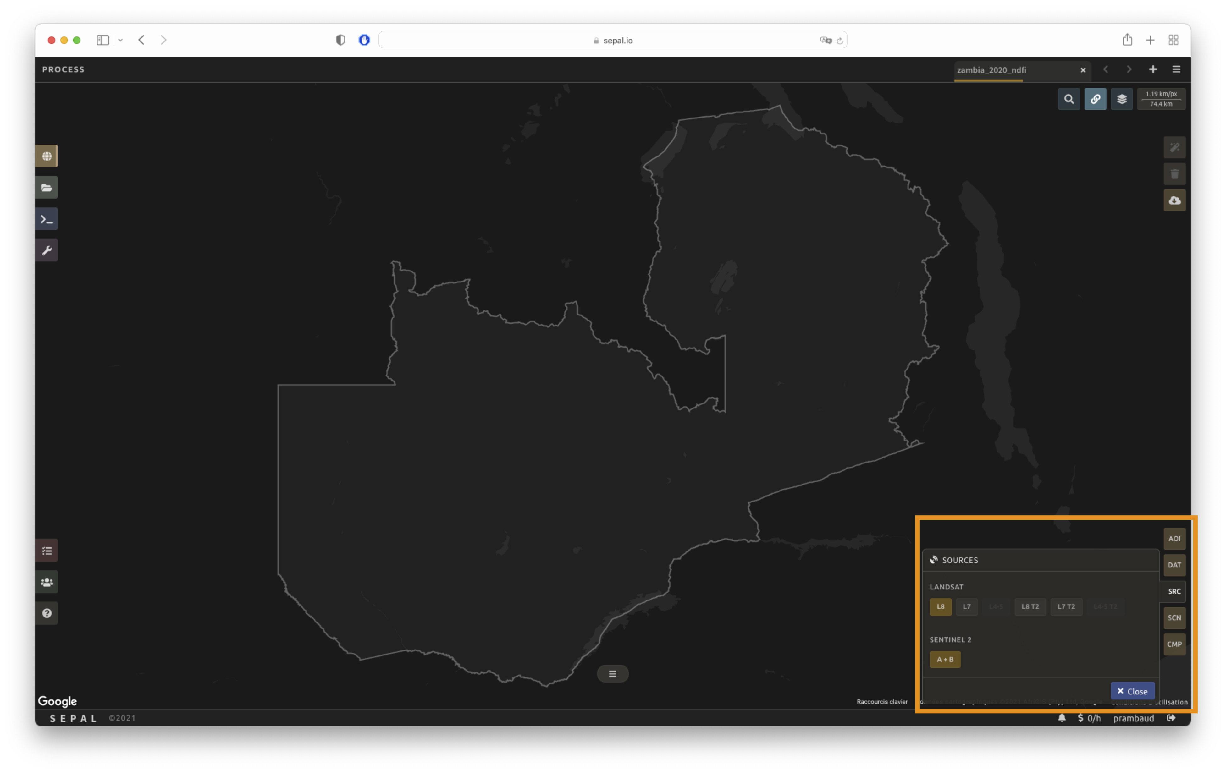
As mentioned in the introduction, a mosaic combines raster datasets that can come from multiple satellite sources. In the SRC tab, select one or more optical data sources to build the mosaic from.
Landsat scenes are distributed in two quality tiers:
Tier 1 holds the scenes with the highest data quality. They are processed to Level-1 Precision Terrain (L1TP), have well-characterized radiometry, are intercalibrated across the different Landsat sensors and are geo-registered within prescribed tolerances (12 m root mean square error [RMSE] or less). Tier 1 scenes are consistent across the full collection and suitable for time-series analysis.
Tier 2 (marked T2) holds scenes that do not meet the Tier 1 criteria, for example because of significant cloud cover, insufficient ground control or systematic-only terrain correction (L1GT/L1GS). They can still be useful; analyze the RMSE and other properties to determine their suitability for your study.
The following optical sources are available (select a link to open the corresponding Google Earth Engine dataset):
L9: Landsat 9 (Tier 1; from 2021).
L8: Landsat 8 (Tier 1; from 2013).
L7: Landsat 7 (Tier 1; from 1999).
L4-5: Landsat 4 combined with Landsat 5 (Tier 1; 1982–2012).
L9 T2, L8 T2, L7 T2, L4-5 T2: the Tier 2 equivalents of the datasets listed above.
S2: Sentinel-2 (Sentinel-2A and Sentinel-2B; from 2015). A wide-swath, high-resolution, multispectral imaging mission supporting Copernicus Land Monitoring studies, including the monitoring of vegetation, soil and water cover, as well as the observation of inland waterways and coastal areas.
Note
SEPAL uses the Landsat Collection 2 archive and the harmonized Sentinel-2 collection.
You can also restrict the imagery with the Max cloud cover % slider: scenes whose cloud cover is higher than this threshold are excluded before the mosaic is built.
To validate your selection, select the Apply button (labelled Done when you first create the recipe through the setup wizard).
Scènes#
Note
Si les données Sentinel et Landsat ont été sélectionnées, vous serez forcé d’utiliser toutes les scènes. Comme le système de tuilage de Sentinel et Landsat est différent, il est impossible de sélectionner des scènes à l’aide de l’outil présenté dans les sections suivantes.
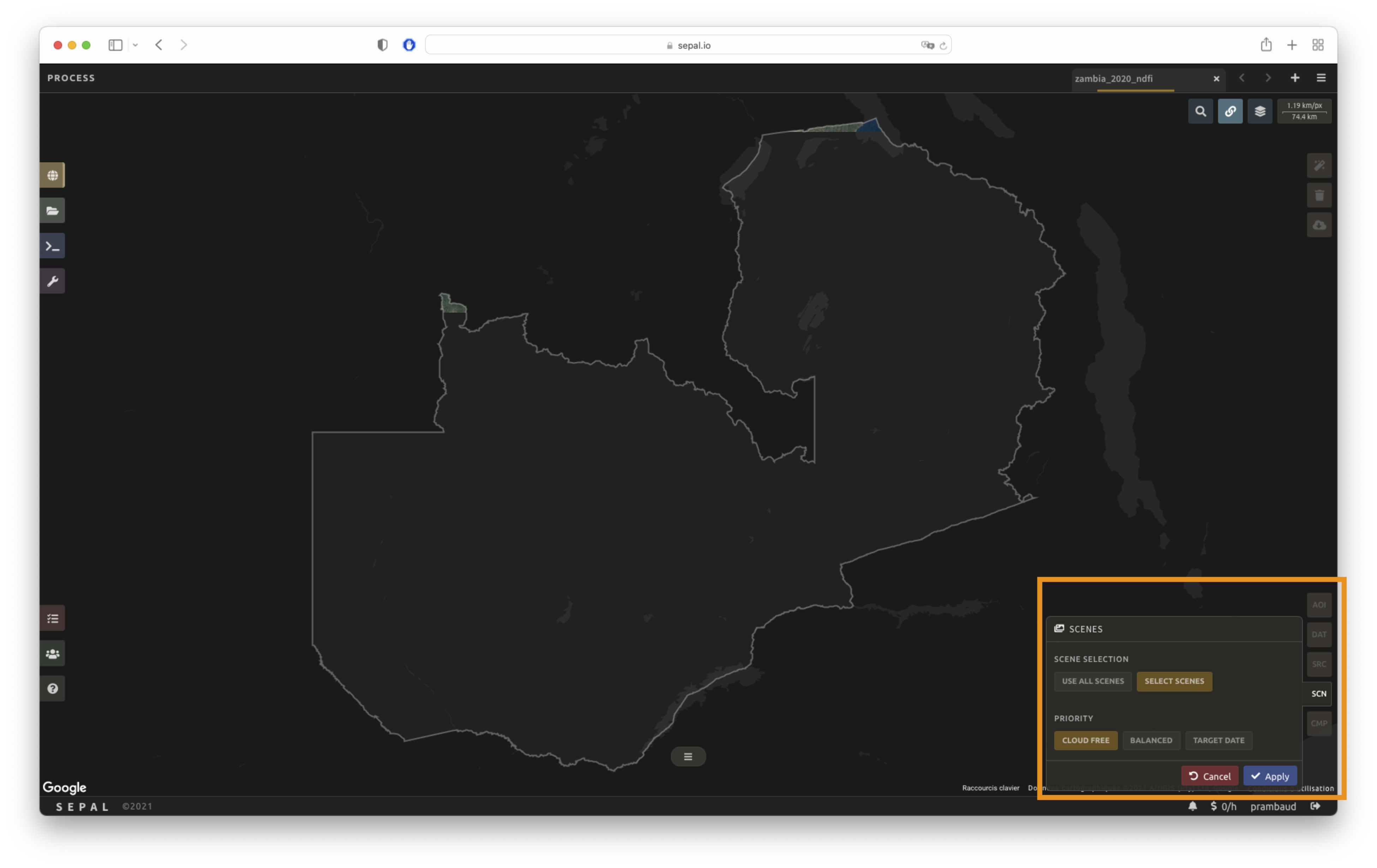
Vous pouvez utiliser plusieurs options pour sélectionner les meilleures scènes de votre mosaïque. Le plus simple est d’utiliser toutes les images disponibles en fonction des paramètres de date. Sélectionnez Utilisez toutes les scènes et toutes les images seront intégrées dans la mosaïque.
Choose Select scenes and pick one of the three available Priority options, based on the needs of your analysis (SEPAL sorts the images available for each tile):
Cloud free: Prioritizes imagery as cloud-free as possible, ignoring the date.
Balanced: Prioritizes imagery that is neither too cloudy nor too far from the target date.
Target date: Prioritizes imagery as close as possible to the target date.
To validate your selection, select the Apply button.
Composite#
The CMP tab controls how the selected scenes are corrected, how clouds and snow are masked, and how the final pixel values are computed. The panel opens in a simple view showing the most common options; select More to reveal the advanced options (and Less to hide them again).
Note
This step is optional. By default, SEPAL applies:
Corrections: SR and BRDF
Masquage des nuages: Modéré
Composition de la méthode: Medoid
The advanced view additionally defaults to no pixel filters, no cloud buffering and snow/ice masking turned on.
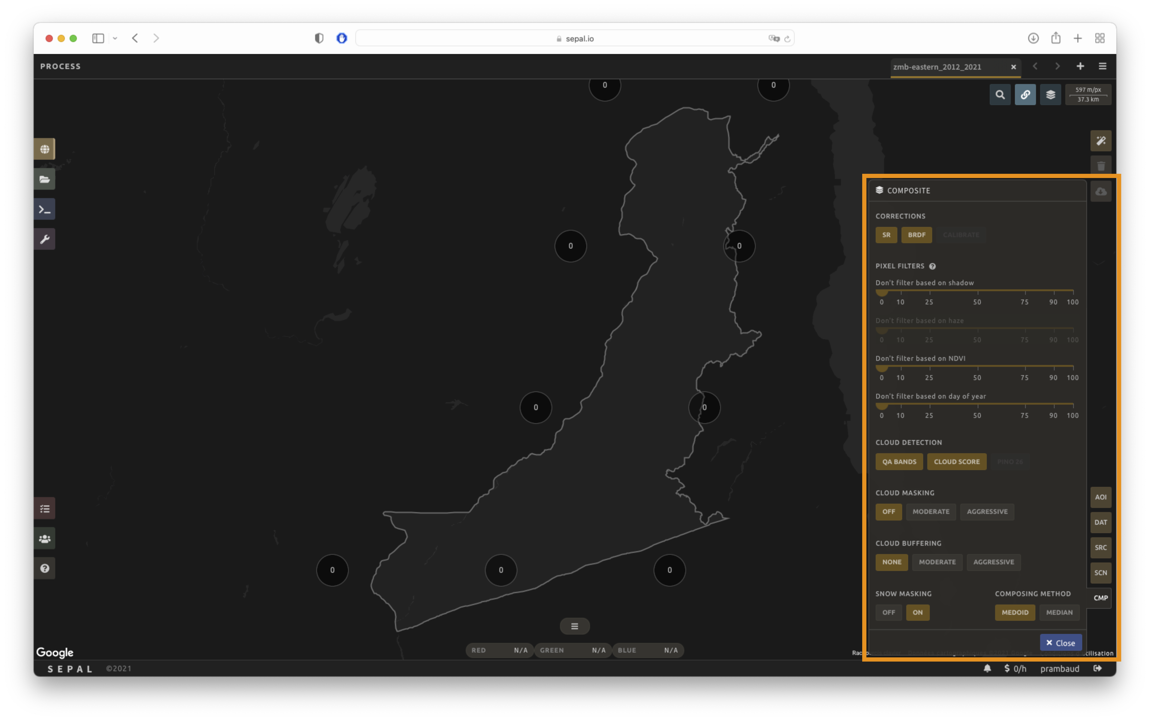
Show the advanced view (opened with More)
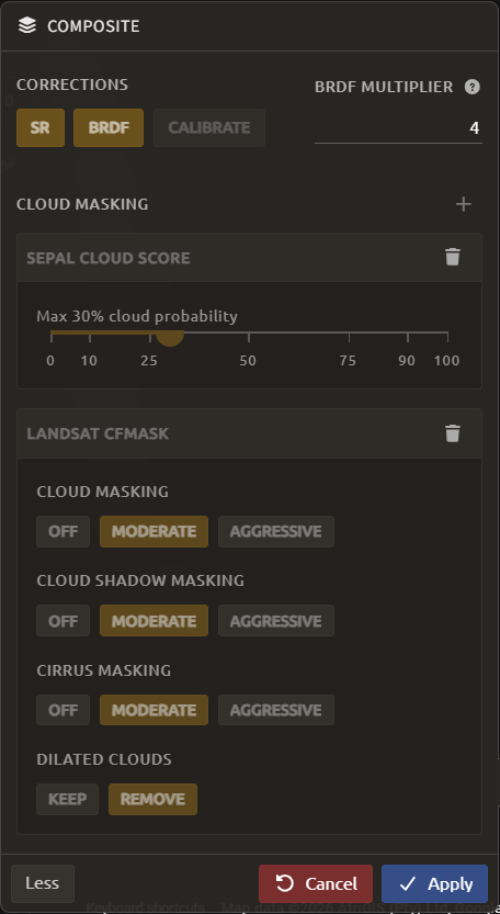
Corrections#
Corrections are applied to the stacked pixels to improve the quality of the mosaic.
SR: Surface reflectance improves comparison between multiple images over the same region by accounting for atmospheric effects such as aerosol scattering and thin clouds, which can help in the detection and characterization of Earth surface change. Top-of-atmosphere (TOA) images are used if not selected.
BRDF: Uses a bidirectional reflectance distribution function (BRDF) model to characterize surface reflectance anisotropy. For a given land area, the BRDF is established based on selected multi-angular observations of surface reflectance. When BRDF is enabled, the advanced view shows a
BRDF Multiplierfield that controls how much correction is applied (values of 3–4 usually work well; lower it if the effect is overcompensated, raise it if it is not compensated enough).Calibrate: Calibrates the bands to improve a cross-sensor mosaic.
Note
Cette option n’est disponible que si :
Landsat and Sentinel-2 data are mixed; and
surface reflectance (SR) correction is disabled.
Masquage des nuages#
Controls how clouds are detected and masked. In the simple view, choose a preset:
Moderate: Relies only on the image source QA bands for cloud masking.
Aggressive: Relies on the image source QA bands together with a cloud-scoring algorithm. This will probably mask out some built-up areas and other bright features.
Custom: Automatically selected (and otherwise disabled) when you fine-tune the individual cloud-masking algorithms in the advanced view.
In the advanced view you can add and configure the individual cloud-masking algorithms with the button. The available algorithms depend on the sources you selected:
SEPAL cloud score: SEPAL’s own cloud-scoring algorithm, with a configurable maximum cloud probability. Always available.
S2 Cloud Score+: Sentinel-2 Cloud Score+, with a maximum cloud probability and a choice of scoring band — cs (instantaneous clear-sky similarity) or cs_cdf (likelihood of being clear over time). Sentinel-2 sources only.
S2 Cloud Probability: the Sentinel-2 cloud-probability dataset, with a configurable maximum cloud probability. Sentinel-2 sources only.
Landsat CFMask: the Landsat CFMask QA bands. You can set
Cloud Masking,Cloud Shadow MaskingandCirrus Maskingeach to Off, Moderate or Aggressive, and choose whether to Keep or Remove dilated clouds. Landsat sources only.Pino 26: the Pan-Tropical Sentinel-2 cloud-detection algorithm developed by Dario Simonetti (for more information, see D. Simonetti [2021]). Only available for a Sentinel-2-exclusive source when SR correction is disabled.
Cloud buffering#
(Advanced view.) When pixels are identified as clouds, SEPAL can also mask a small buffer around them to prevent hazy pixels at the borders of clouds from being included in the mosaic.
Note
Buffering is done at the pixel level, so using this option significantly increases the creation time of the mosaic.
None: Doesn’t use cloud buffering.
Moderate: Masks an additional 120 m around each larger cloud.
Aggressive: Masks an additional 600 m around each larger cloud.
Snow/ice masking#
(Advanced view.) Defines how snowy or icy pixels are masked.
On: Masks snow. This tends to leave some pixels with shadowy snow.
Off: Doesn’t mask snow. Note that some clouds might get misclassified as snow; therefore, disabling snow masking might lead to cloud artifacts.
Masked out pixels#
(Advanced view.) Controls whether a pixel can end up completely masked when every available acquisition is cloudy and/or snowy.
Prevent: Prevents pixels from being completely masked out, keeping the best available (possibly cloudy/snowy) value.
Allow: Allows pixels to be completely masked out, leaving holes in the mosaic where no clear observation exists.
Filtres des pixels#
(Advanced view.) Add filters with the button to remove pixels from the stack before compositing. Each filter excludes a percentage of the stack (set with a slider, defaulting to 50%); removing low-quality pixels improves the quality of the mosaic.
Note
Each filter is applied iteratively (e.g. if the normalized difference vegetation index [NDVI] is already filtering all pixels but one, there will be nothing left in the stack to be filtered by date).
Note as well that adding filters significantly increases the creation time of the mosaic.
Shadow: Excludes the selected percentage of pixels with the most shadow.
Haze: Excludes the selected percentage of pixels with the most haze. Only available when SR correction is disabled.
NDVI: Excludes the selected percentage of pixels with the lowest NDVI.
Date: Excludes the selected percentage of pixels farthest from the target date.
Sentinel-2 overlap#
(Advanced view; shown only when Sentinel-2 is selected.) Sentinel-2 acquisitions overlap both between orbits and between neighbouring tiles, which can result in duplicated observations.
Orbit Overlap: Keep the overlap between Sentinel-2 orbits (more data, better models) or Remove it.
Tile Overlap: Keep the overlap between Sentinel-2 tiles, Quick remove most of it, or Remove all of it. Removing overlap adds an extra preprocessing step.
Méthode de composition#
After filtering the stack of pixels, the composing method defines how the final pixel value is extracted.
Medoid: Uses the pixel closest to the median value. As a real pixel from the stack, the final value embeds metadata (e.g. the date of observation).
Median: Uses the computed median value. If no pixel matches this value, the pixel will not embed any metadata. It tends to produce smoother mosaics.
Analyse#
After selecting the parameters, you can start interacting with the scenes and begin the analysis.
In the upper-right corner, three tabs are available, which allow you to customize the mosaic scene selection and export the final result:
: auto-select scenes
: clear selected scenes
: retrieve mosaic
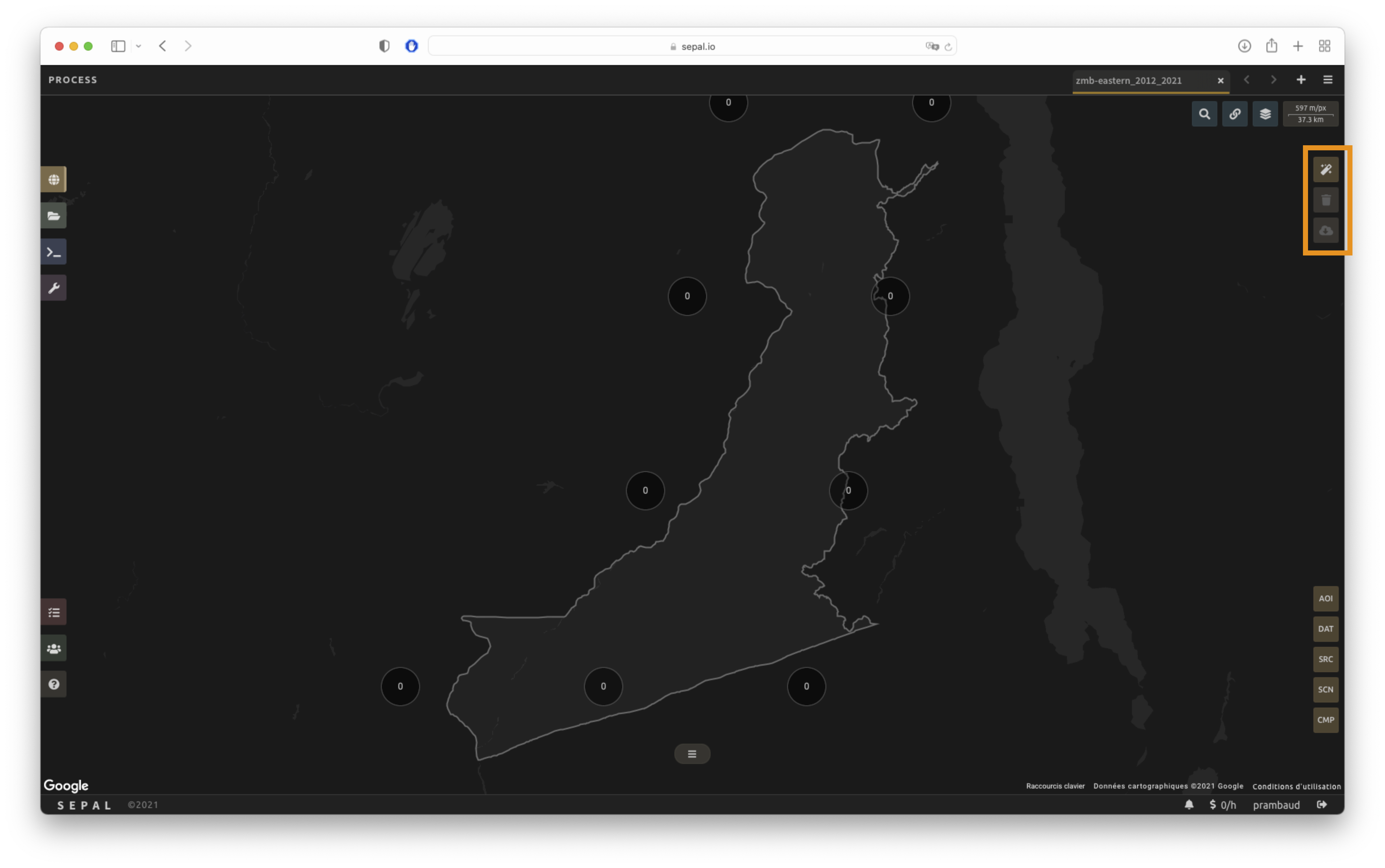
Note
If you have not selected the option Select scenes in the SCN tab, the button will be disabled and the scene areas will be hidden as no scene selection needs to be performed (see those with a number in a circle on the previous screenshot).
If you can’t see the image scene area, you probably have selected a small AOI. Zoom out on the map and you will see the number of available images in the circles.
Sélectionner les scènes#
To create a mosaic, select the scenes that will be used to compute each pixel value of the mosaic. SEPAL provides a user-friendly interface that will guide you through the selection process. You don’t have to select the stack for every pixel; instead, SEPAL will clip the AOI in smaller pieces called Tiles. These tiles correspond to the native tiling system of your dataset and are displayed on the map with circled numbers in their centroid. Each number corresponds to the number of scenes available to build the mosaic tile. Hover over these circles to see the tile boundaries appear.
Note
Landsat and Sentinel datasets have a different grid system, which is why the selection process cannot be used if you have selected both of these datasets. If you have an idea related to the user interface (UI) that could make them work together, let us know in our issue tracker.
Auto-select scene#
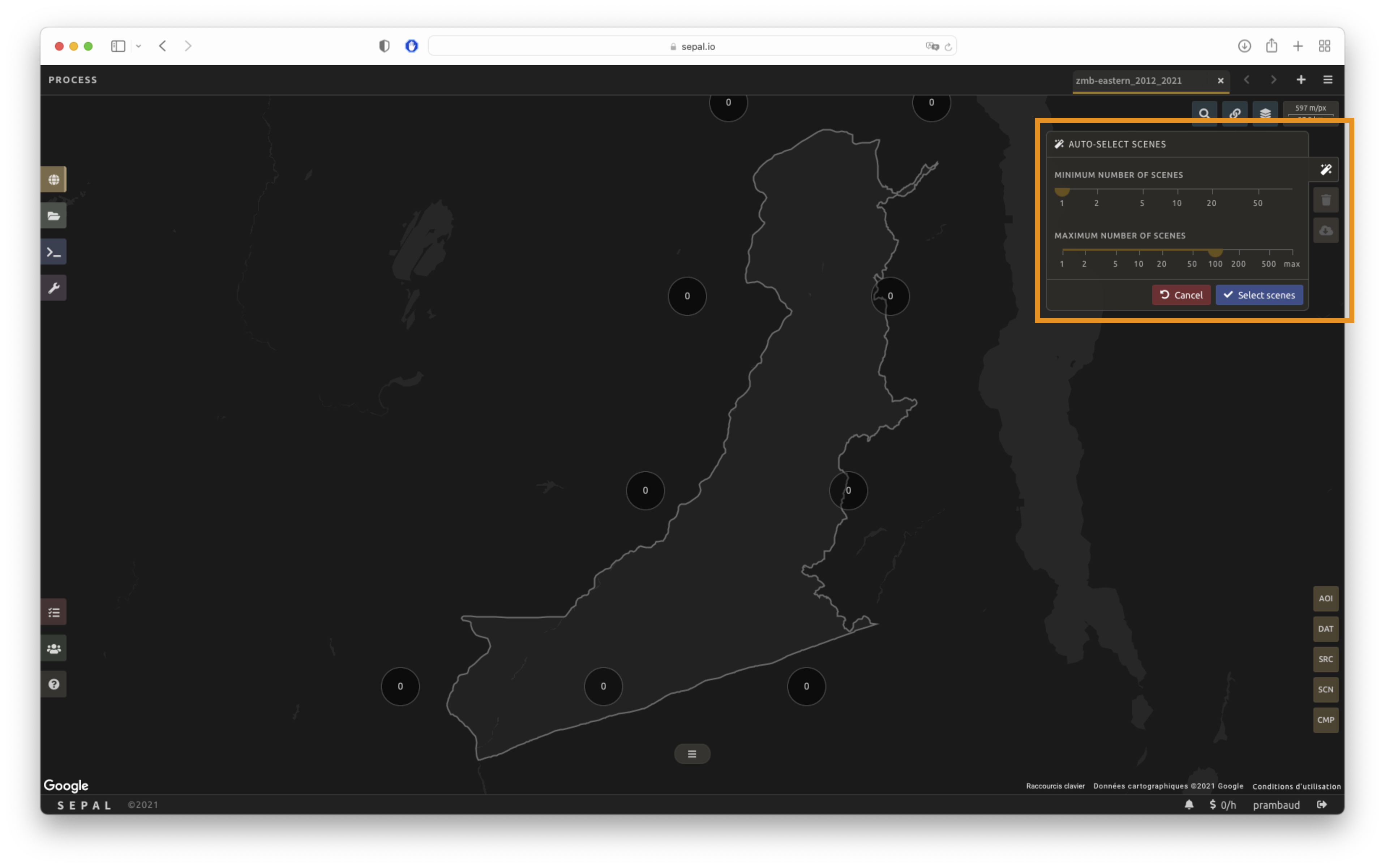
Selecting the tab will open the Auto-selection pane.
Move the sliders to set the Minimum number of scenes and the Maximum number of scenes SEPAL should select in a tile. Then, select the Select scenes button to apply the auto-select method.
SEPAL will use the priority defined in the SCN tab to order the scene and collect the optimal number for your request.
Note
The result is never perfect but can be used as a starting point for the manual selection of scenes.
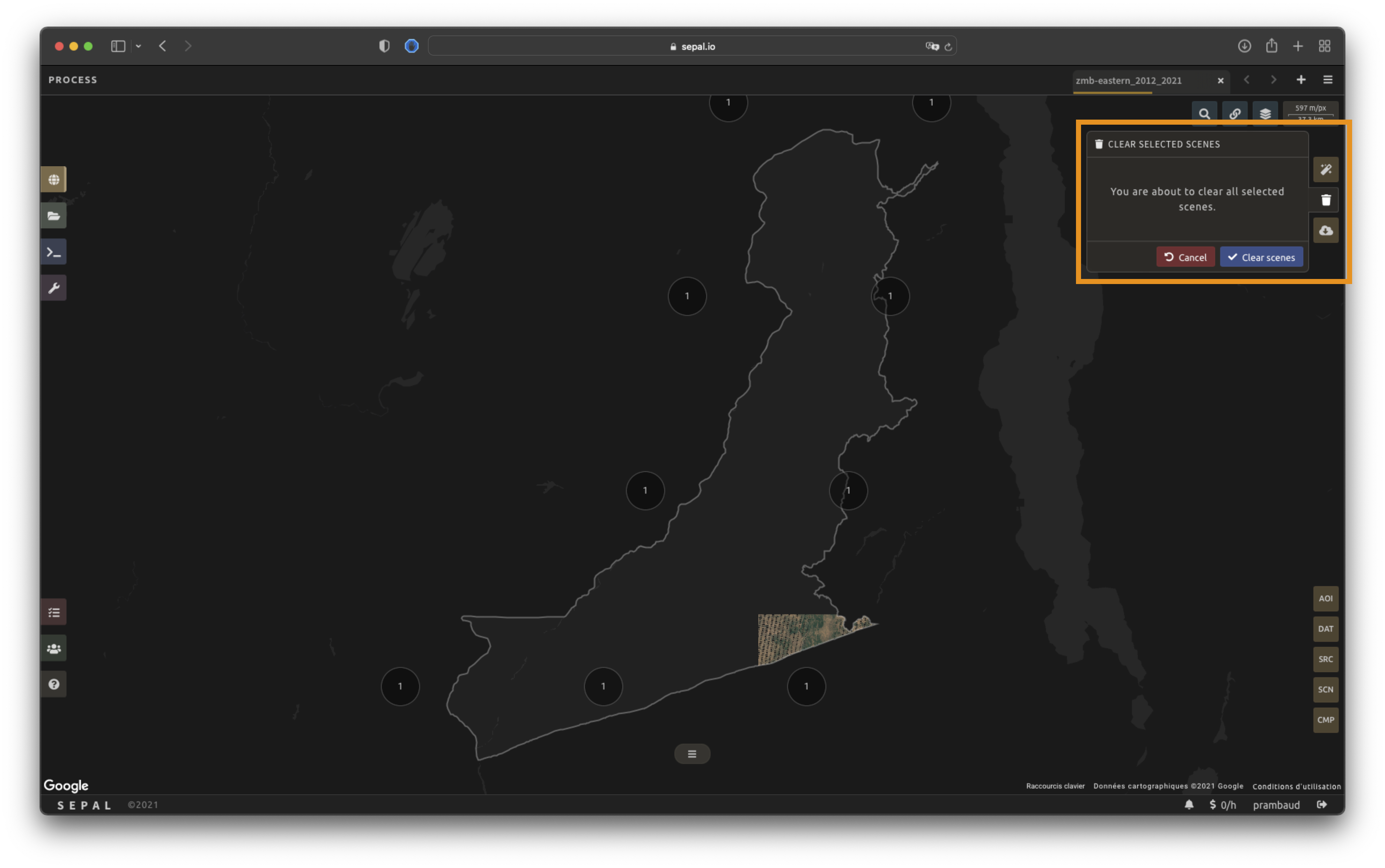
Clear all scenes#
If at least one scene is selected, the tab will be available. Select it to open the Clear pane.
Select Clear scenes to remove all manually and automatically selected scenes.
Manual selection#
To open the Scene selection menu, hover over a tile circled-number and select it (1). The window will be divided into two sections:
Available scene (2): All the available scenes according to the parameters you selected. These scenes are ordered using the
priorityparameter you set in the SCN tab.Selected scenes (3): The scenes that are currently selected.
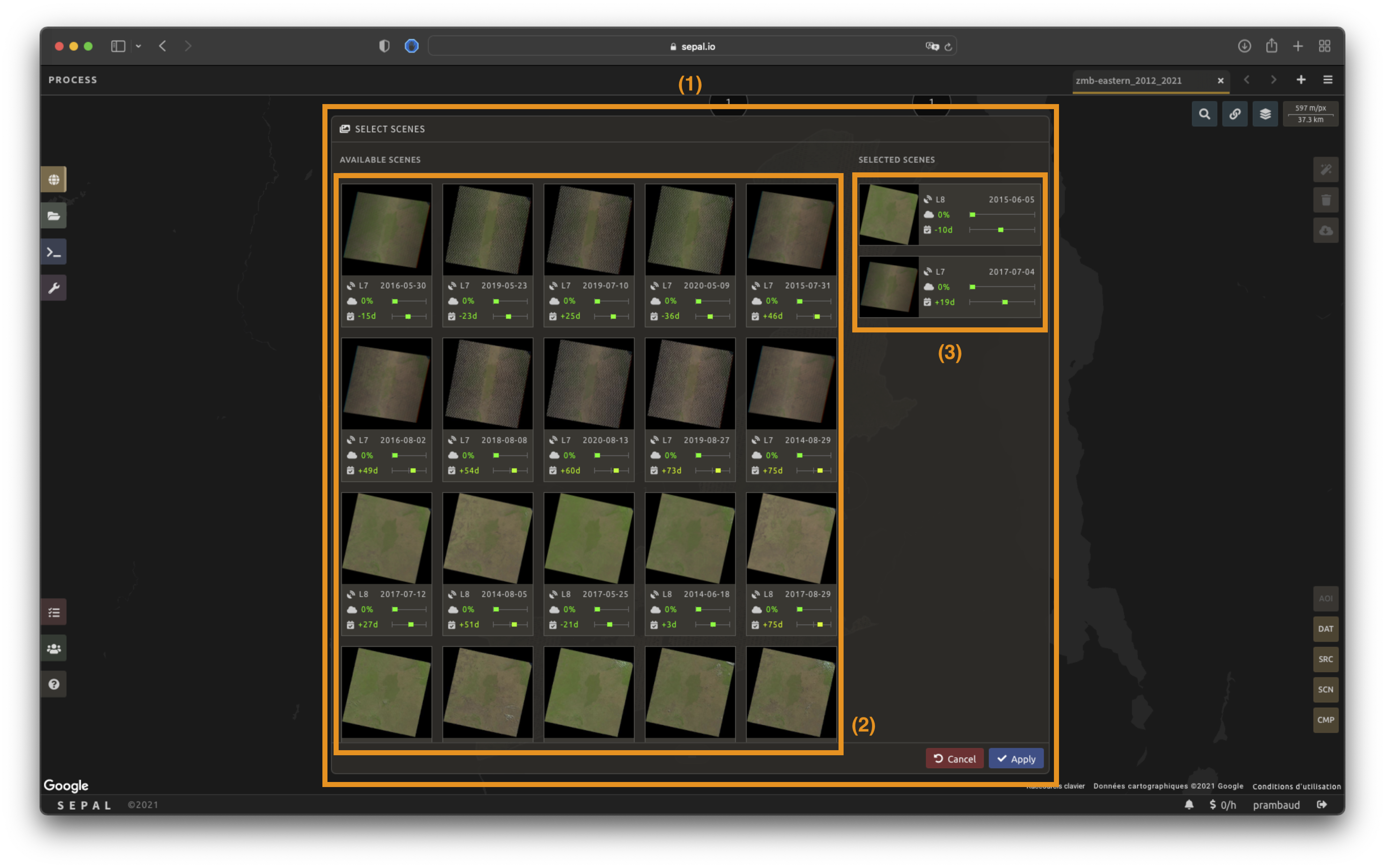
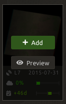
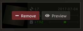
Each thumbnail represents a scene of the tile stack. You have the option to include them in the mosaic. The scenes located on the left side are the Available scenes; the Selected scenes are on the right side. In both cases, the following information can be found on the thumbnail:
A small preview of the scene in the red, green, blue (true-colour) band combination.
The exact date in YYYY-MM-DD of the scene.
The satellite name .
The cloud coverage of the scene in percent and its position in the stack values .
The distance from target day in days within the season and its position in the stack values .
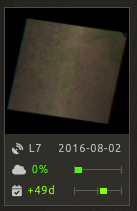
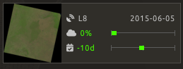
You can decide to move the scene to the Selected scene area by selecting Add or moving it back to the Available scene pane by selecting Remove.
Astuce
Scenes are moved from one side to the other so they are not duplicated and cannot be selected twice. Be careful if your connection is slow; wait for the thumbnail to move before clicking again (if you click too fast, you could select two different images instead of one).
Once you are happy with your selection, select the Apply button to close the window and use the selected scenes to compute the mosaic on this tile. When the window is closed, SEPAL resets the rendering of all tiles.
Retrieve#
Important
You cannot export a recipe as an asset or a .tif file without a small computation quota. If you are a new user, see Gérer vos ressources.
Selecting the tab will open the Retrieve pane where you can select the exportation parameters.
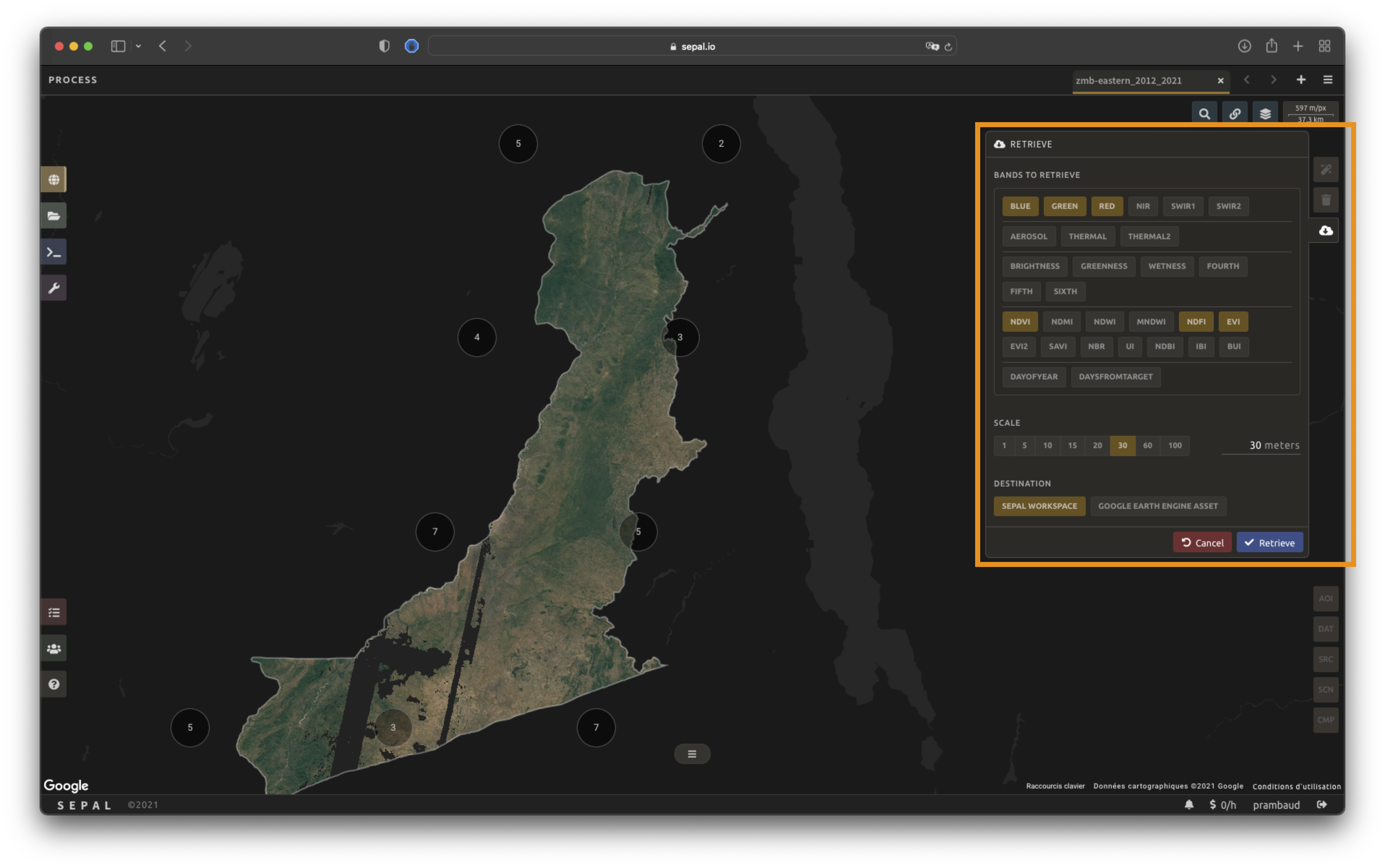
Bands#
You need to select the band(s) to export with the mosaic. There is no maximum number of bands, but exporting useless bands will only increase the size and time of the output. To discover the full list of available bands with SEPAL, see Optical Satellite bands, transformations, and indices.
Astuce
There is no fixed rule to the band selection. Each index is more adapted to a set of analyses in a defined biome. The knowledge of the study area, the evolution expected and the careful selection of an adapted band combination will improve the quality of downstream analysis.
Dates#
dayOfYear: the Julian calendar date (day of the year)
daysFromTarget: the distance to the target date within the season in days
Note
These metadata bands are only available when the Medoid composing method is used (the Median method produces artificial pixels that carry no metadata).
Échelle#
You can set a custom scale for exportation by selecting a value in metres (m) (note that requesting a smaller resolution than the images” native resolution will not improve the quality of the output – just its size – keep in mind that the native resolution of Sentinel data is 10 m, while Landsat is 30 m).
Récupérer vers#
Choose a single destination for the export:
SEPAL workspace: the image is written to your SEPAL files in
.tifformat (by default in theDownloadsfolder).Google Earth Engine asset: the image is exported to your GEE account as an asset. You can export it either as a single Image or as an Image collection (tiled, which is better suited to large exports), and set its sharing to Private or Public.
Google Drive: the image is exported to the Google Drive of the connected Google account.
Note
The Google Earth Engine asset and Google Drive destinations are only displayed when a Google account is connected to SEPAL. If they are missing, please refer to Connect SEPAL to GEE.
Select Retrieve to start the export process.
Statut d’exportation#
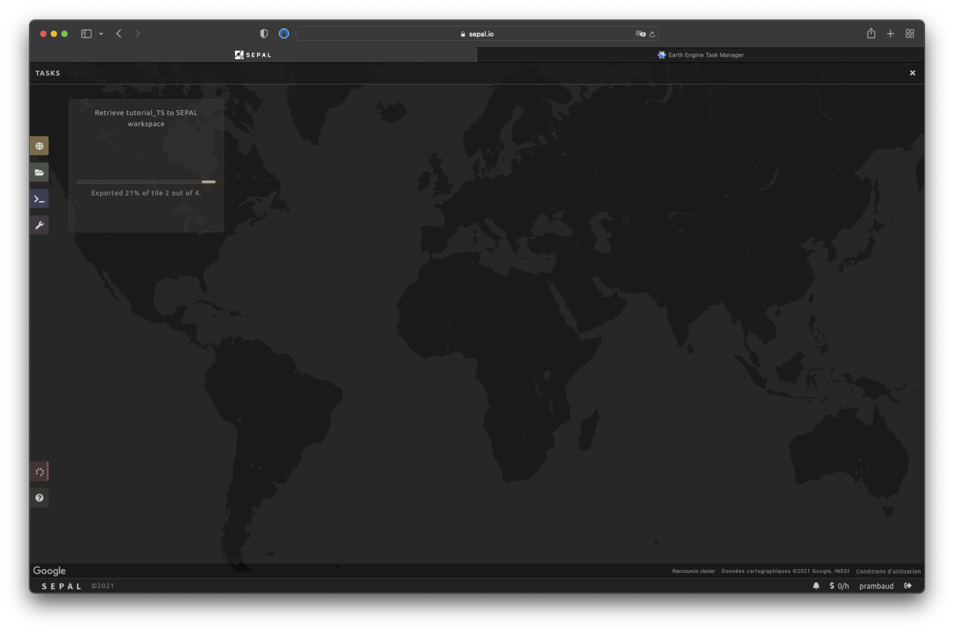
In the Tasks tab (lower-left corner using the or buttons, depending on the loading status), you will see the list of the different loading tasks. The interface will provide you with information about task progress and display an error if the exportation has failed.
Si vous n’êtes pas satisfait de la façon dont nous présentons les informations, la tâche peut également être surveillée en utilisant le Gestionnaire de tâches GEE.
Astuce
Cette opération fonctionne entre les serveurs GEE et SEPAL en arrière-plan. Vous pouvez fermer la page SEPAL sans arrêter le processus.
Lorsque la tâche est terminée, le cadre sera affiché en vert, comme indiqué sur la deuxième image ci-dessous.

Accès#
Une fois le processus de téléchargement terminé, vous pouvez accéder aux données dans vos dossiers SEPAL. Les données seront stockées dans le dossier Downloads en utilisant le format suivant :
.
└── downloads/
    └── <MO name>/
        ├── <MO name>_<gee tile id>.tif
        ├── <MO name>_<gee tile id>.tif
        ├── ...
        ├── <MO name>_<gee tile id>.tif
        └── <MO name>_<gee tile id>.vrt
Note
Understanding how images are stored in an optical mosaic is only required if you want to manually use them. The SEPAL applications are bound to this tiling system and can digest the information for you.
Les données sont stockées dans un dossier en utilisant le nom de la mosaïque optique telle qu’elle a été créée dans la première section de cet article. Comme le nombre de données est spatialement trop grand pour être exporté en même temps, les données sont divisées en morceaux plus petits et réunies dans un fichier <MO name>_<gee tile id>.vrt.
Astuce
The full folder with a consistent tree folder is required to read the .vrt
Important
Now that you have exported the optical mosaic to your SEPAL workspace, it can be downloaded to your computer using file exchange options or used in other SEPAL workflows.