

Classification#
Build supervised classifications of mosaic images to create easy-to-use user interfaces with the Classification recipe
Présentation#
With this recipe, SEPAL helps users build supervised classifications of any mosaic image. It is built on top of the most advanced tools available on Google Earth Engine (GEE) – including the classifiers CART, RandomForest, NaiveBayes and SVM – allowing users to create an easy-to-use user interface to:
select an image to classify;
définir la table de classe ; et
ajouter des données d’entrainement à partir de sources externes et de sélection à la volée.
In combination with other tools of SEPAL, the Classification recipe can help you provide accurate land-use maps, without writing a single line of code.
Commencer#
Once the Classification recipe is selected, SEPAL will show the recipe process in a new tab (see 1 in figure below); the Image selection window will appear in the lower right (2).
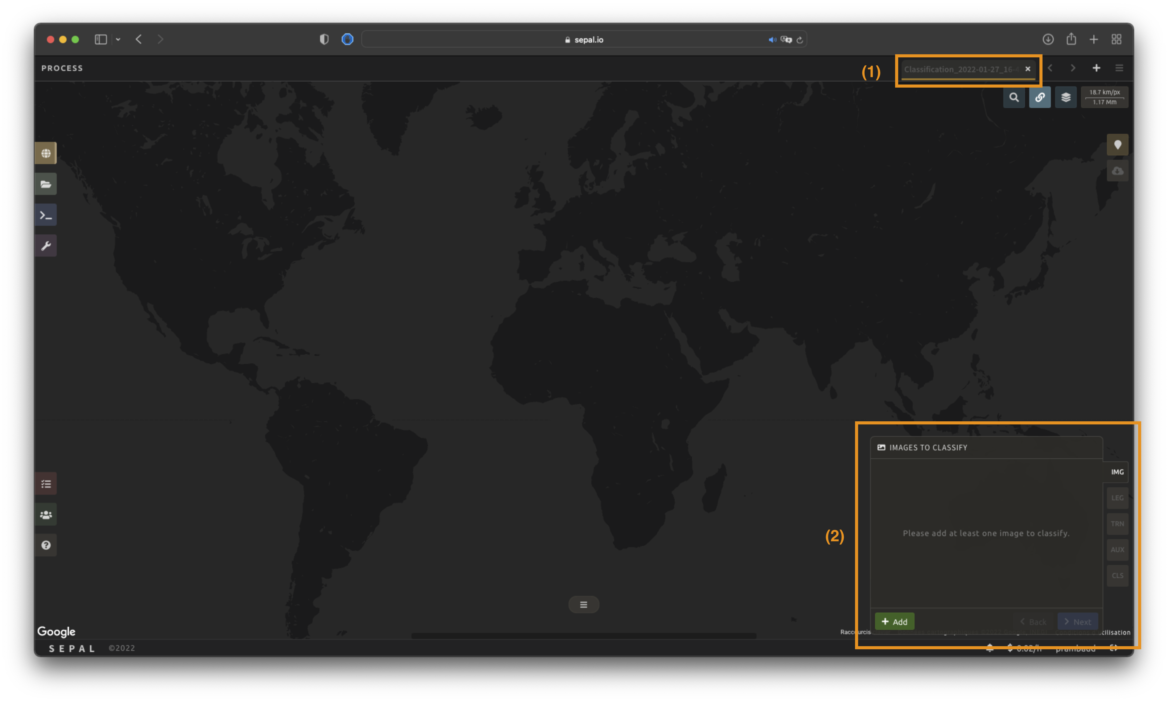
La première étape est de changer le nom de la recette. Ce nom sera utilisé pour identifier vos fichiers et recettes dans les dossiers SEPAL. Utilisez la convention la mieux adaptée à vos besoins. Double-cliquez simplement sur l’onglet et entrez un nouveau nom. Il sera par défaut à Classification_<timestamp>.

Note
L’équipe SEPAL recommande d’utiliser la convention suivante : <image_name>_<classification>_<measures>.
Paramètres#
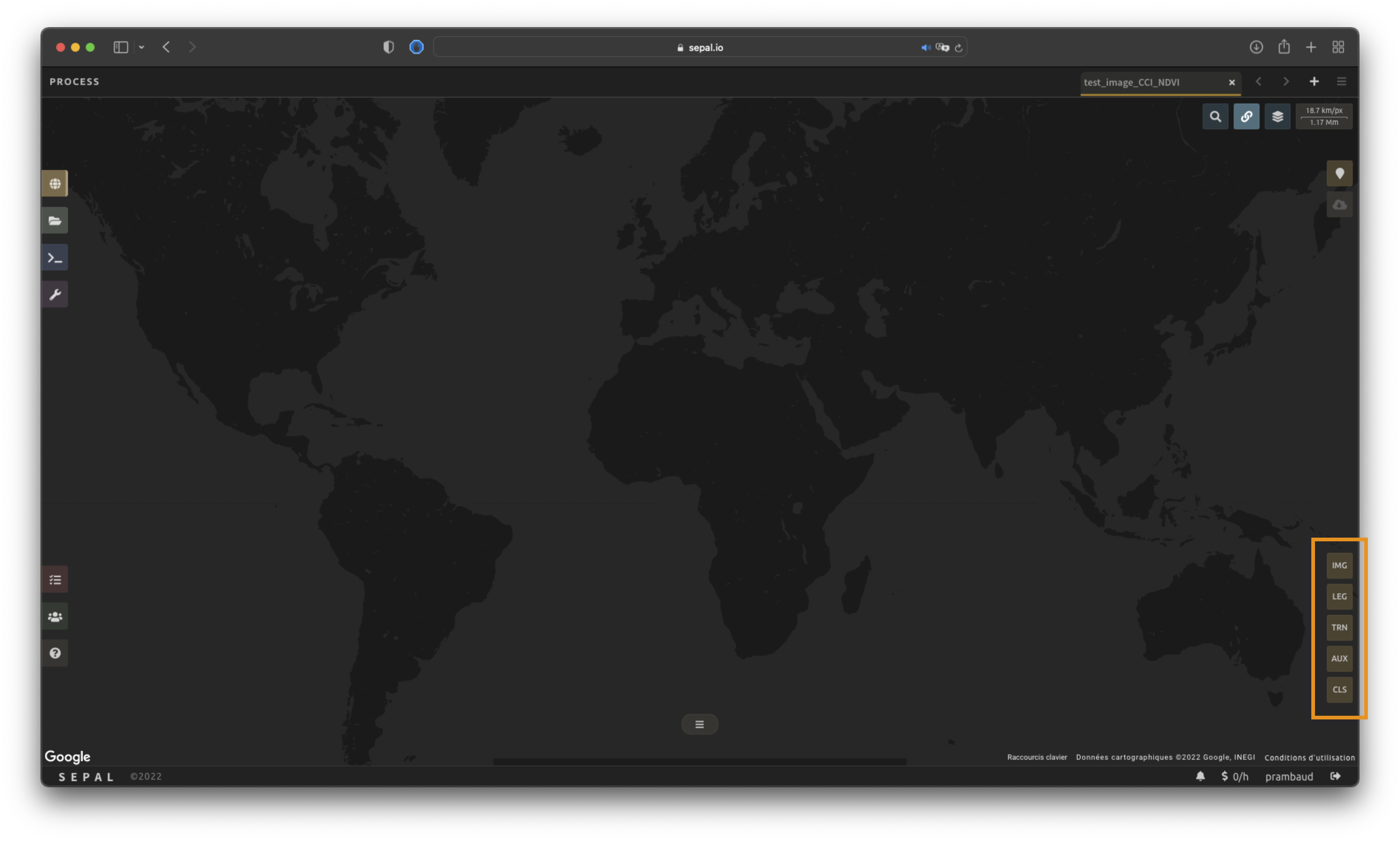
Dans le coin inférieur droit, les cinq onglets suivants sont disponibles, vous permettant de personnaliser la série temporelle selon vos besoins:
IMG: image to classify
LEG: legend of the classification system
TRN: training data of the model
AUX: auxiliary global dataset to use in the model
CLS: classifier configuration
Sélection de l’image#
La première étape consiste à sélectionner les bandes d’images sur lesquelles appliquer le classificateur. Le nombre de bandes sélectionnées (c’est-à-dire les images) n’est pas limité.
Note
Gardez à l’esprit que l’augmentation du nombre de bandes à analyser améliorera le modèle mais ralentira le rendu de l’image finale.
Note
If multiple images are selected, all selected images should overlap. If masked pixels are found in one of the bands, the classifier will mask them.
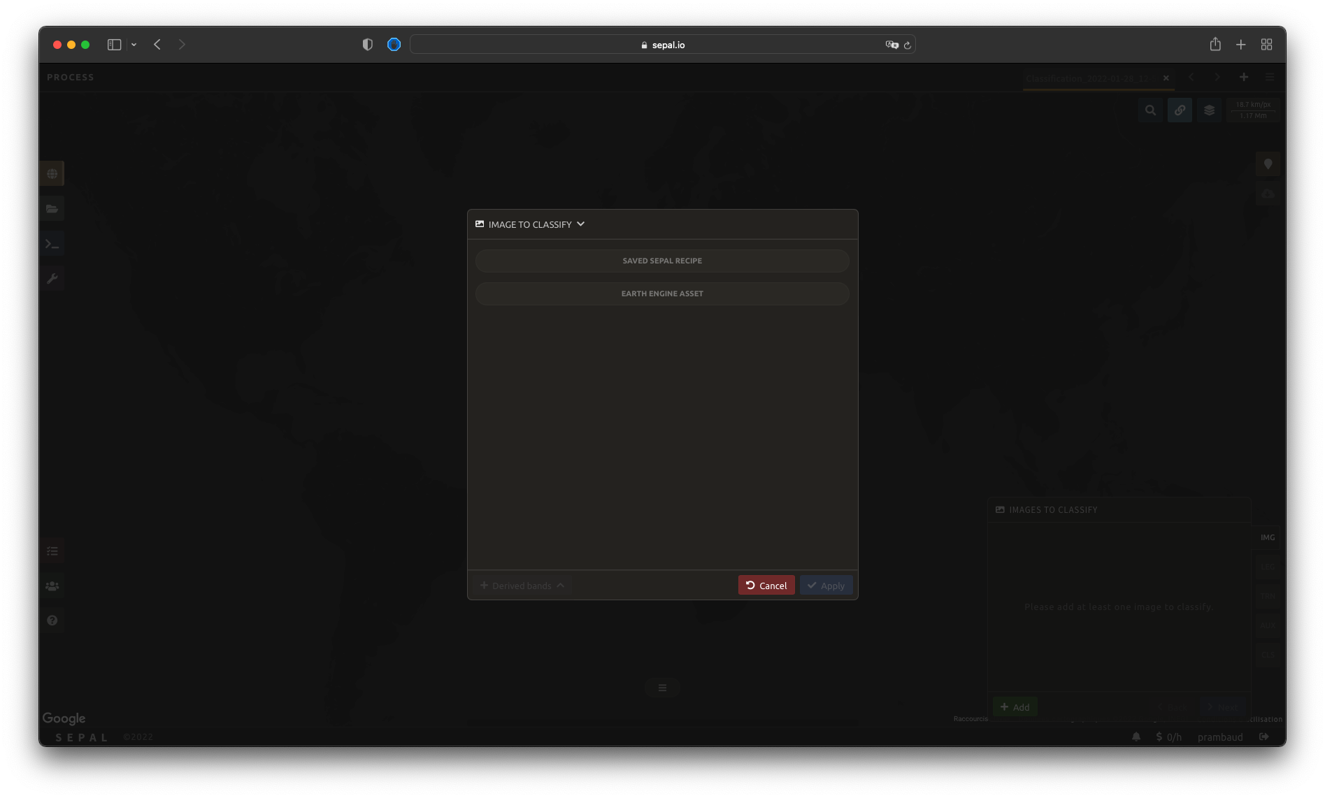
Select Add. The following screen should be displayed:
Type d’image#
Les utilisateurs peuvent sélectionner des images provenant d’une recette existante ou d’un asset GEE exporté (voir avantages et inconvénients ci-dessous). Les deux devraient être un ee.Image, plutôt qu’une série temporelle ou ee.ImageCollection.
Recette existante:
Avantages :
all of the computed bands from SEPAL can be used; and
any modification to the existing recipe will be propagated in the final classification.
Inconvénients :
the initial recipe will be computed at each rendering step, slowing down the classification process and potentially breaking on-the-fly rendering due to GEE timeout errors.
Asset GEE:
Avantages :
can be shared with other users; and
the computation will be faster, as the image has already been exported.
Inconvénients :
only the exported bands will be available; and
the
Imageneeds to be re-exported to propagate changes.
Les deux méthodes se comportent de la même manière dans l’interface.
Sélectionnez des bandes#
Astuce
For this example, we will use a public asset created with the Optical mosaic tool from SEPAL. It’s a Sentinel-2 mosaic of Eastern Province in Zambia during the dry season from 2012 to 2020. Multiple bands are available.
Utilisez le nom d’actif suivant si vous voulez reproduire notre flux de travail: projects/sepal-cookbook/assets/classification/zmb-eastern_2012_2021
Bandes spectrales#
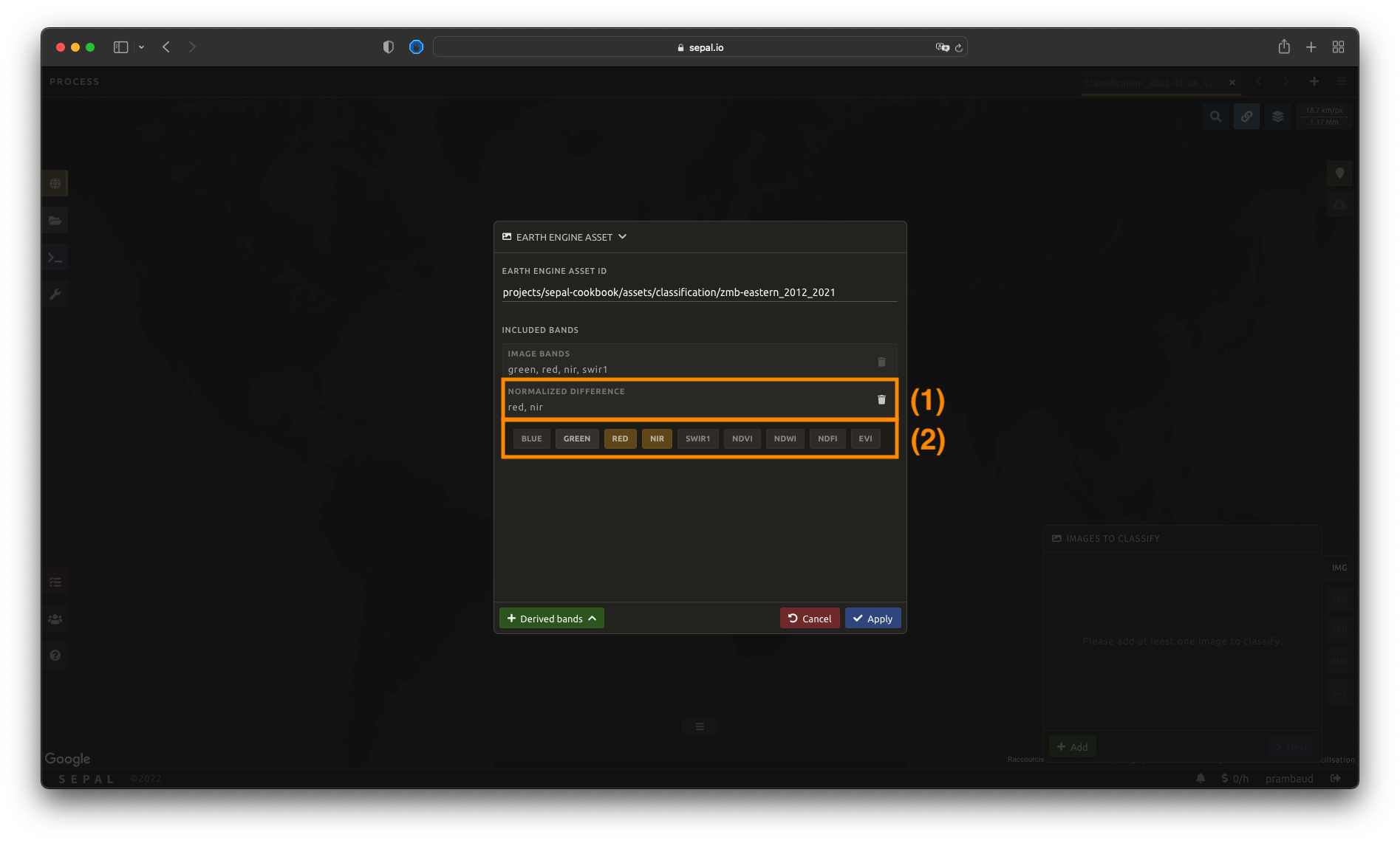
Once an asset has been selected, SEPAL will load its bands in the interface. You can use any band that is native to the image as input for the classification process. Simply click on the band name to select them. The selected bands are summarized in the expansion panel title (1) and displayed in gold in the pane content (2).
Dans cet exemple, nous avons sélectionné les éléments suivants :
rougenirswirvert

Bandes dérivées#
L’analyse ne se limite pas à des bandes natives disponibles ; SEPAL peut également construire des bandes dérivées supplémentaires à la volée.
Select Derived bands at the bottom of the pop-up window and select the deriving method. This will add a a new panel to the expansion panel with the selected method name (1). The selected method will be applied to the selected bands.
Note
Si plus de deux bandes sont sélectionnées, l’opération sera appliquée au produit cartésien des bandes. Si vous sélectionnez des bandes \(A\), \(B\) et \(C\), et appliquez les bandes dérivées de Différence, vous ajouterez trois bandes à votre analyse :
\(A - B\)
\(A - C\)
\(B - C\)
Note
You should notice that in the figure, we compute the normalized difference between nir and red (i.e. the NDVI). It is also pre-computed in the Indexes derived bands.
Once image selection is complete, select Apply and the pop-up window will close. The images and bands will be displayed in the IMG panel in the lower-right corner of the screen. By selecting the button, you will remove the image and its band from the analysis altogether.
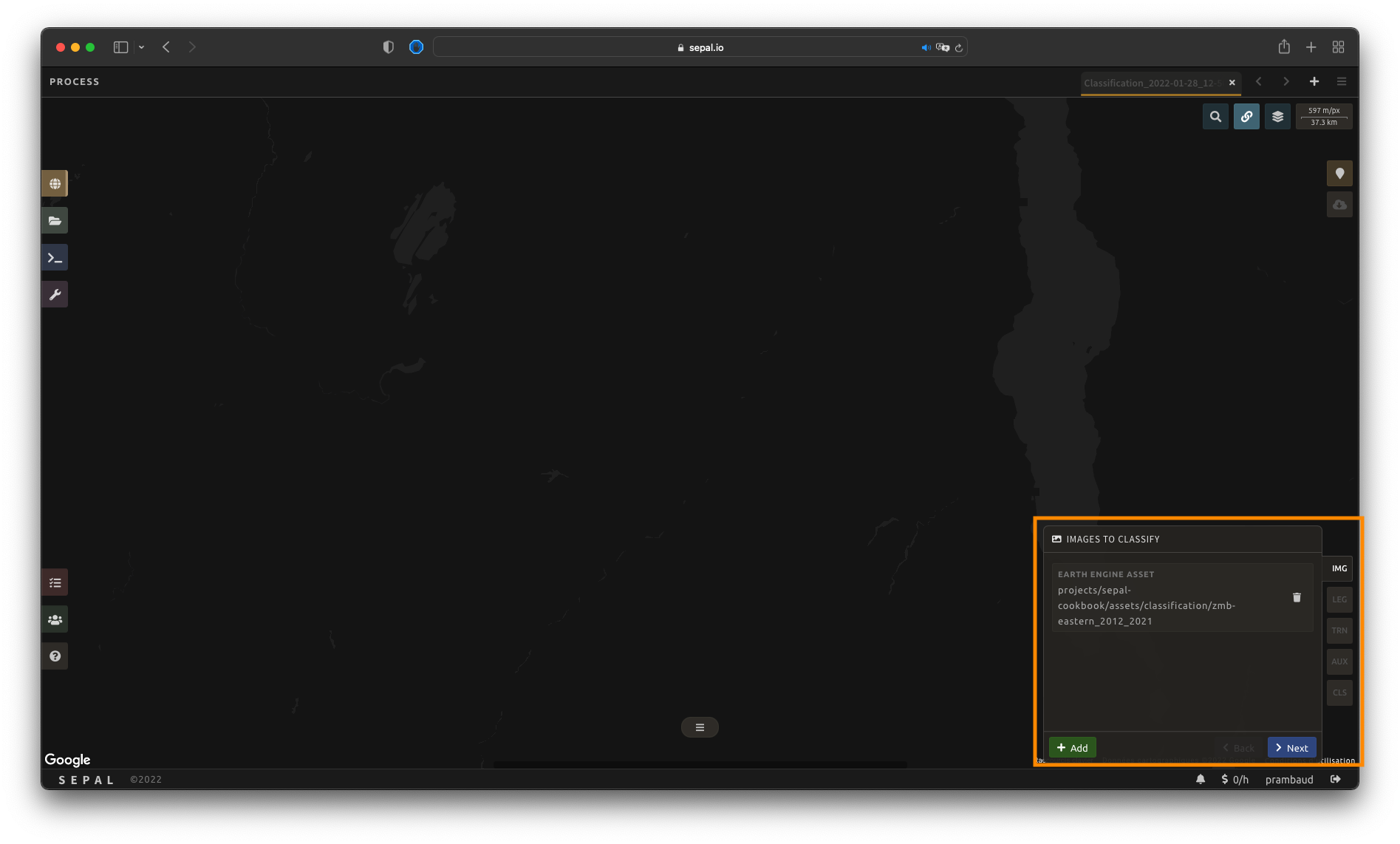
From there, select Next to continue to the next step.
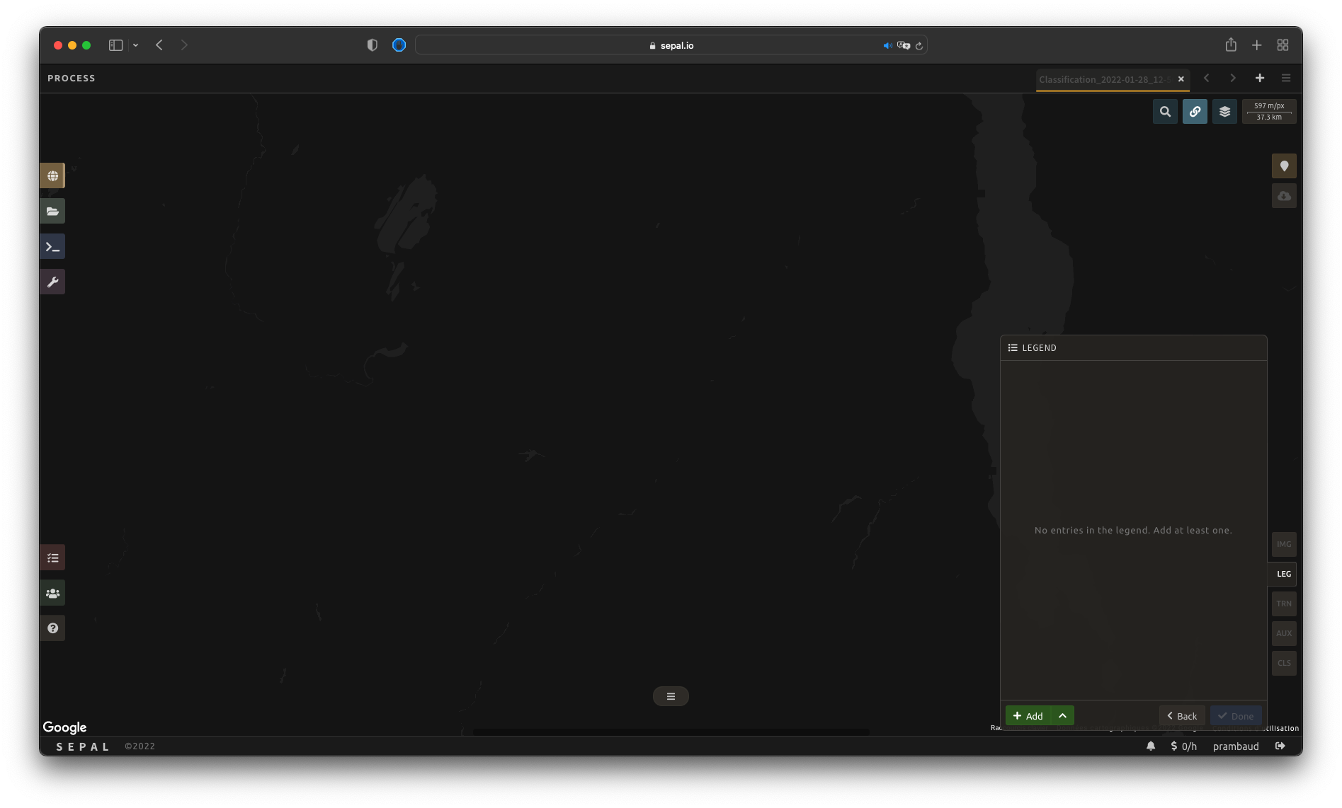
Configuration de la légende#
Dans cette étape, l’utilisateur spécifiera la légende qui doit être utilisée dans l’image de sortie classifiée. Toute classification catégorielle qui associe une valeur entière à un nom de classe fonctionnera. SEPAL fournit plusieurs façons de créer et de personnaliser une légende.
Important
Les légendes créées ici sont entièrement compatibles avec d’autres fonctionnalités de SEPAL, y compris les applications.
Légende manuelle#
La première et la plus naturelle façon de construire une légende est de le faire à partir de zéro.
Select Add to add a new class to your legend.
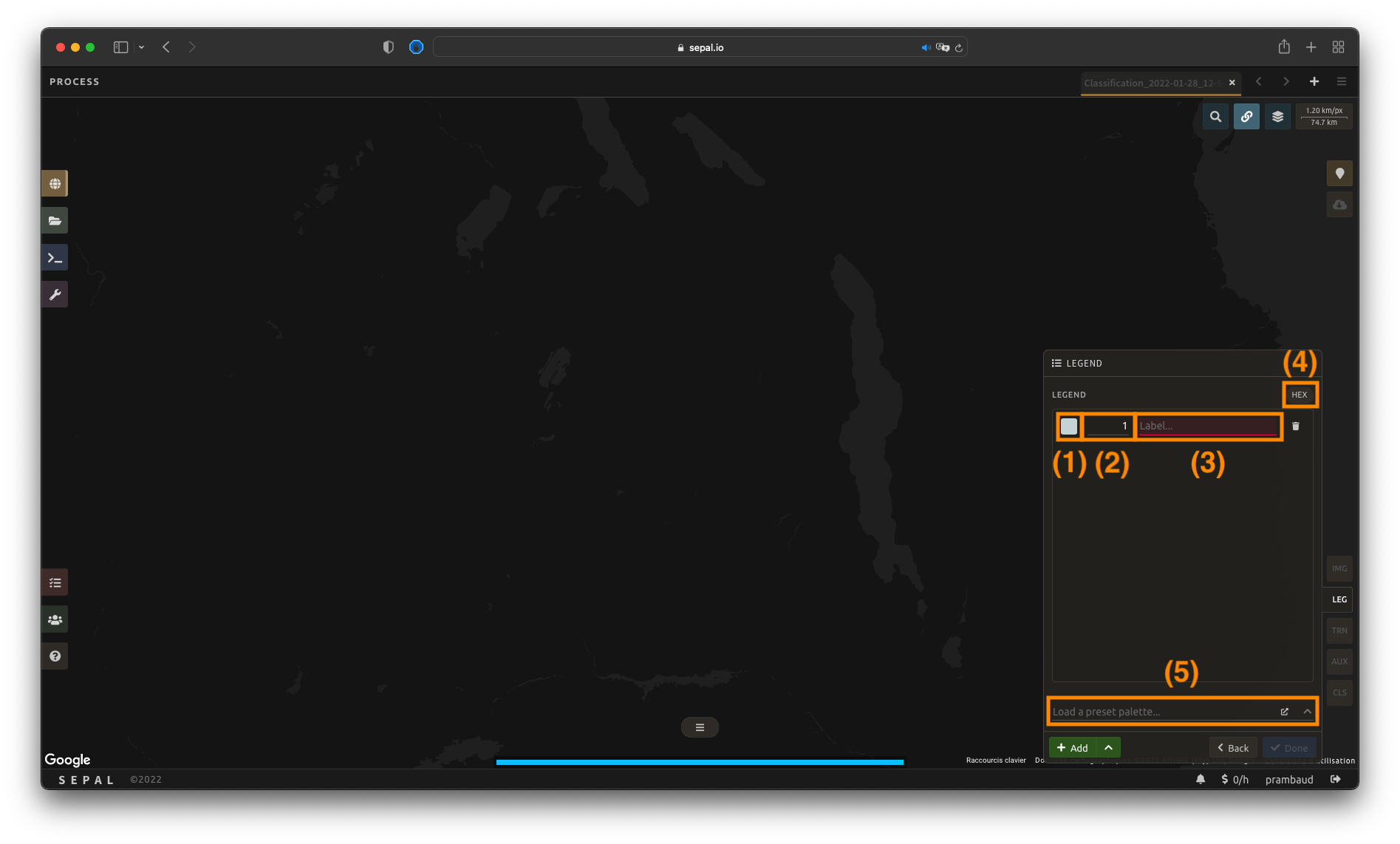
Une classe est définie par trois éléments clés :
Couleur (1) : Sélectionnez le petit carré de couleur pour ouvrir le sélecteur de couleur et choisissez n’importe quelle couleur (la couleur doit être unique).
Valeur (2): Sélectionnez n’importe quelle valeur entière (la valeur doit être unique).
Classe (3): Insérer une description de classe (ne peut pas être vide).
Select the Add button again to add an extra class line. The button can be used to remove a specific line.
Astuce
Sélectionnez HEX (4) pour afficher la valeur hexadécimale de la couleur sélectionnée. Il peut également être utilisé pour insérer une palette de couleurs connue en utilisant ses valeurs.
If multiple classes are created and you are not sure which one to use, you can apply colors to them by selecting a preselected color-map (5). They are provided by the GEE community and will be applied to every existing class in your panel.
Importer une légende#
Si vous avez déjà un fichier décrivant votre légende, vous pouvez l’utiliser plutôt que d’identifier chaque élément de légende individuellement. Votre légende doit être enregistrée au format .csv et contenir les informations suivantes :
color (stored as a hexadecimal value [e.g. #FFFF00] or in three columns [red, blue, green]);
valeur (stockée en tant qu’entier) ; et
classe (stocké sous forme de chaine de caractères).
Note
The column names will help SEPAL predict information, but are not compulsory.
For example, a .csv file containing the following information is fully qualified to be used in SEPAL:
code,class,color
10,Tree cover,#006400
20,Shrubland,#ffbb22
30,Grassland,#ffff4c
40,Cropland,#f096ff
50,Built-up,#fa0000
60,Bare,#b4b4b4
70,Snow,#f0f0f0
80,Water,#0064c8
90,Herbaceous wetland,#0096a0
95,Mangroves,#00cf75
100,Moss,#fae6a0
Alternatively, a file containing the following information – including RGB-defined colors – is also acceptable:
code,class,red,blue,green
10,Tree cover,0,100,0
20,Shrubland,255,187,34
30,Grassland,255,255,76
40,Cropland,240,150,255
50,Built-up,250,0,0
60,Bare,180,180,180
70,Snow,240,240,240
80,Water,0,100,200
90,Herbaceous wetland,0,150,160
95,Mangroves,0,207,117
100,Moss,250,230,160
Une fois que le fichier de légende entièrement qualifié a été préparé sur votre ordinateur, sélectionnez et ensuite Importer à partir de CSV, qui ouvrira une fenêtre pop-up où vous pouvez glisser-déposer le fichier ou le sélectionner manuellement à partir des fichiers de votre ordinateur.
As shown in the following image, you can then select the columns that are defining your .csv file (select Single column for hexadecimal-defined colors and Multiple columns for RGB-defined colors).
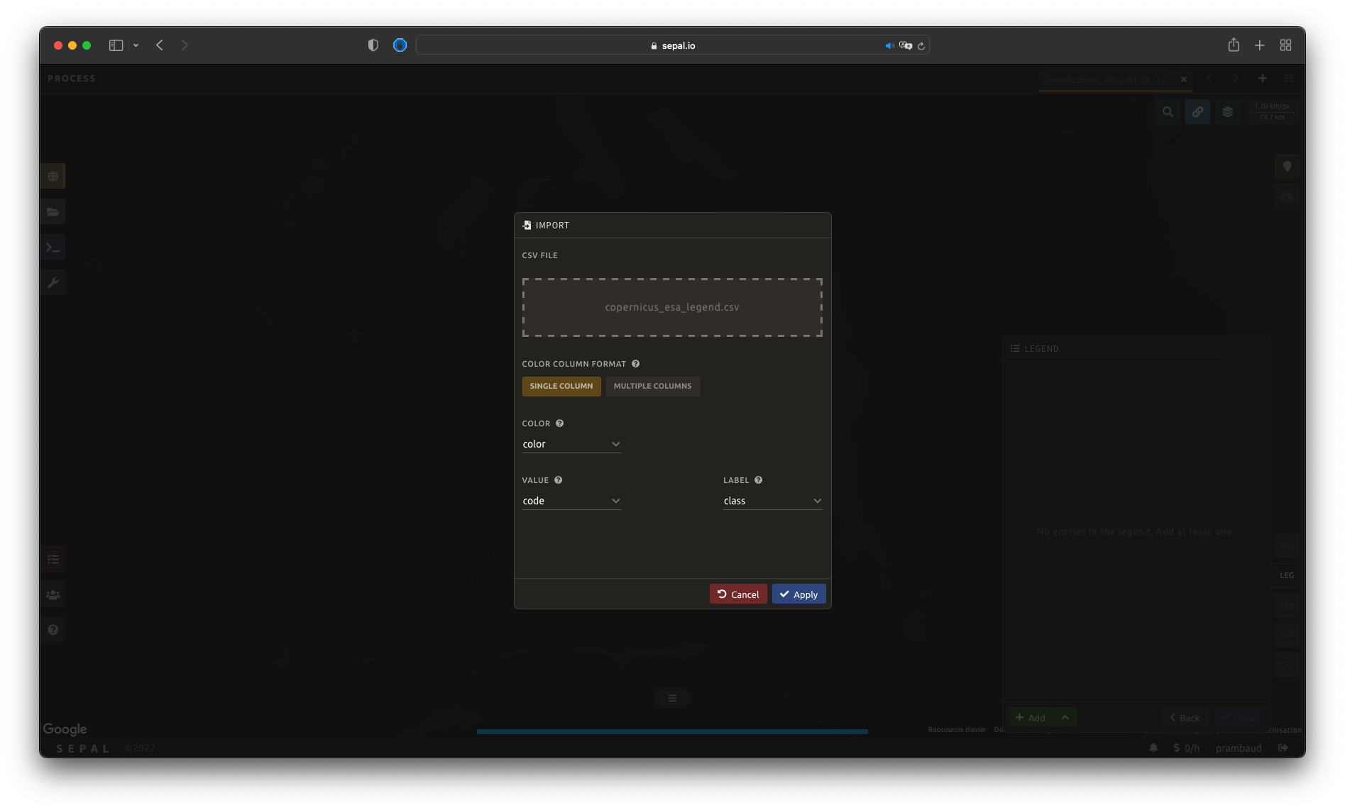
Select Apply to validate your selection. The classes will be added to the legend panel and you’ll be able to modify the legend using the parameters presented in the previous subsection.
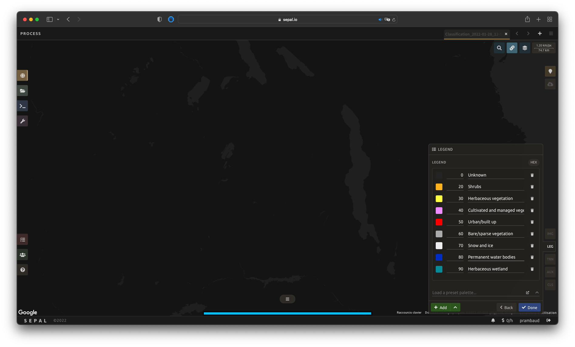
Select Done to validate this step.
Every pane should be closed; the colors of the legend should now be displayed at the bottom of the map. No classification is performed, as we didn’t provide any training data. Nevertheless, this step is the last mandatory step for setting parameters. Training data can be added using the on-the-fly training functionality.
Export legend#
Once your legend is validated, select the and then Export as CSV.
A file will be downloaded to you computer named <recipe_name>_legend.csv, which will contain the legend information in the following format:
color,value,label
#006400,10,Tree cover
...
Select training data#
Note
This step is not mandatory.
Two inputs are required to create the classification output:
pixel values (e.g. bands) to classify; and
training data to set up the classification model.
This menu will help the user manage the training data of the model used. To open it, select TRN in the lower-right side of the window.
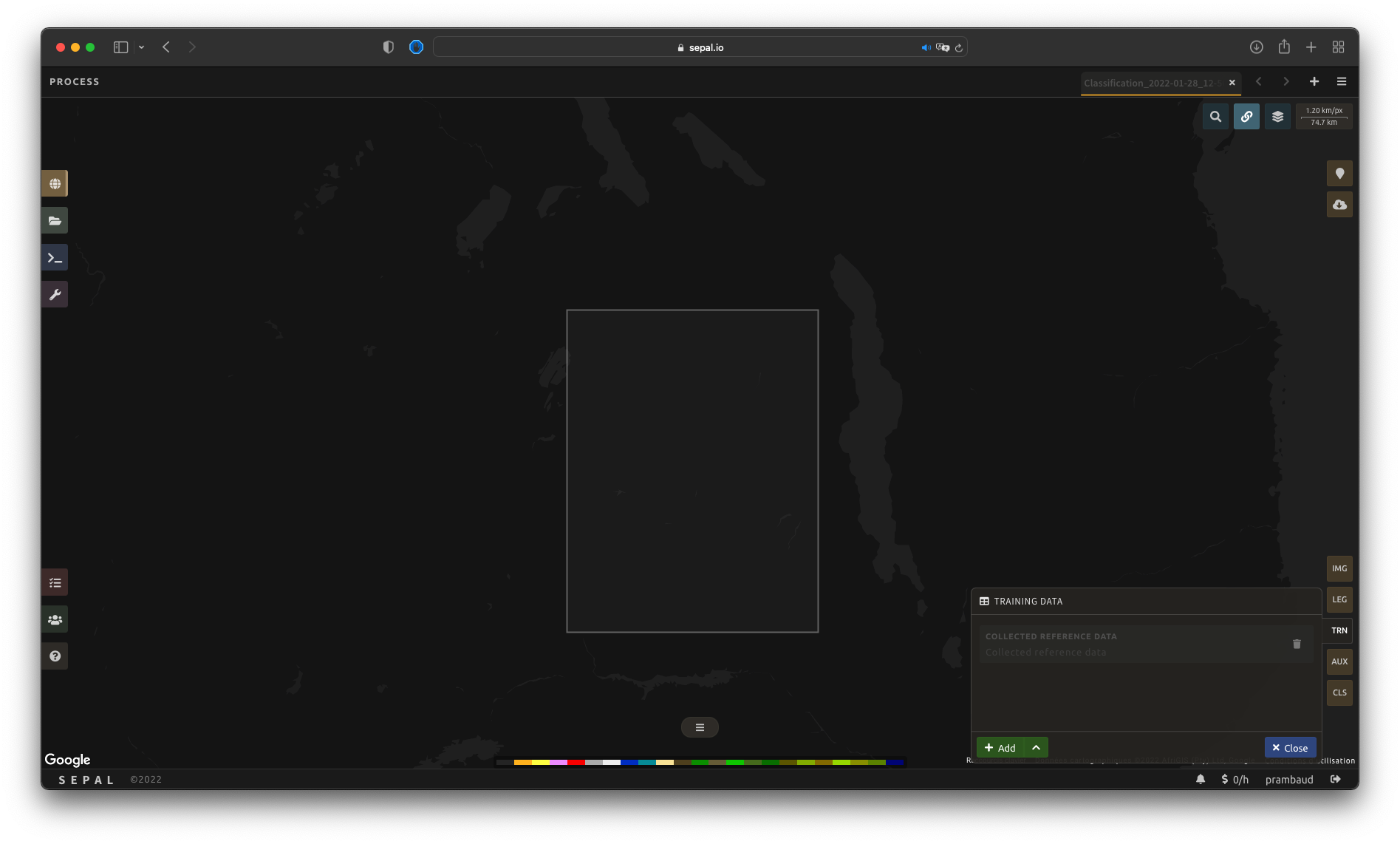
Collected reference data#
Collected reference data are data selected on the fly by the user. The workflow will be explained later in the documentation.
In this pane, this type of data can be managed by the user. The data appear as a pair, associating coordinates to a class value, which will be used to create training data in the classification model.
If you’re satisfied with the current selection and you want to share the data with others, select and then Export reference data to csv. A file will be created and sent to your computer, named <recipe_name>_reference_data.csv. It will embed all of the gathered point data using the following convention:
XCoordinate,YCoordinate,class
32.77189961605467,-11.616264558754402,80
...
If you are not satisfied with the selected data, select and then Clear collected reference data to remove all collected data from the analysis.
Astuce
A confirmation pop-up window should prevent you from accidentally deleting everything.
Existing training data#
Instead of collecting all data by hand, SEPAL provides numerous ways to include already existing training data into your analysis. The data can be from multiple formats and will be included in the model to improve the quality of the final map.
Note
The imported files can use an extended version of the legend provided in the previous step, but to avoid unexpected behaviour, at least one of the classes of your legend and the provided training data need to match.
Note
If the added training data are outside of the image to classify, they will have no impact on the final result (with the exception of the SEPAL recipe).
To add new data, select Add and choose the type of data to import:
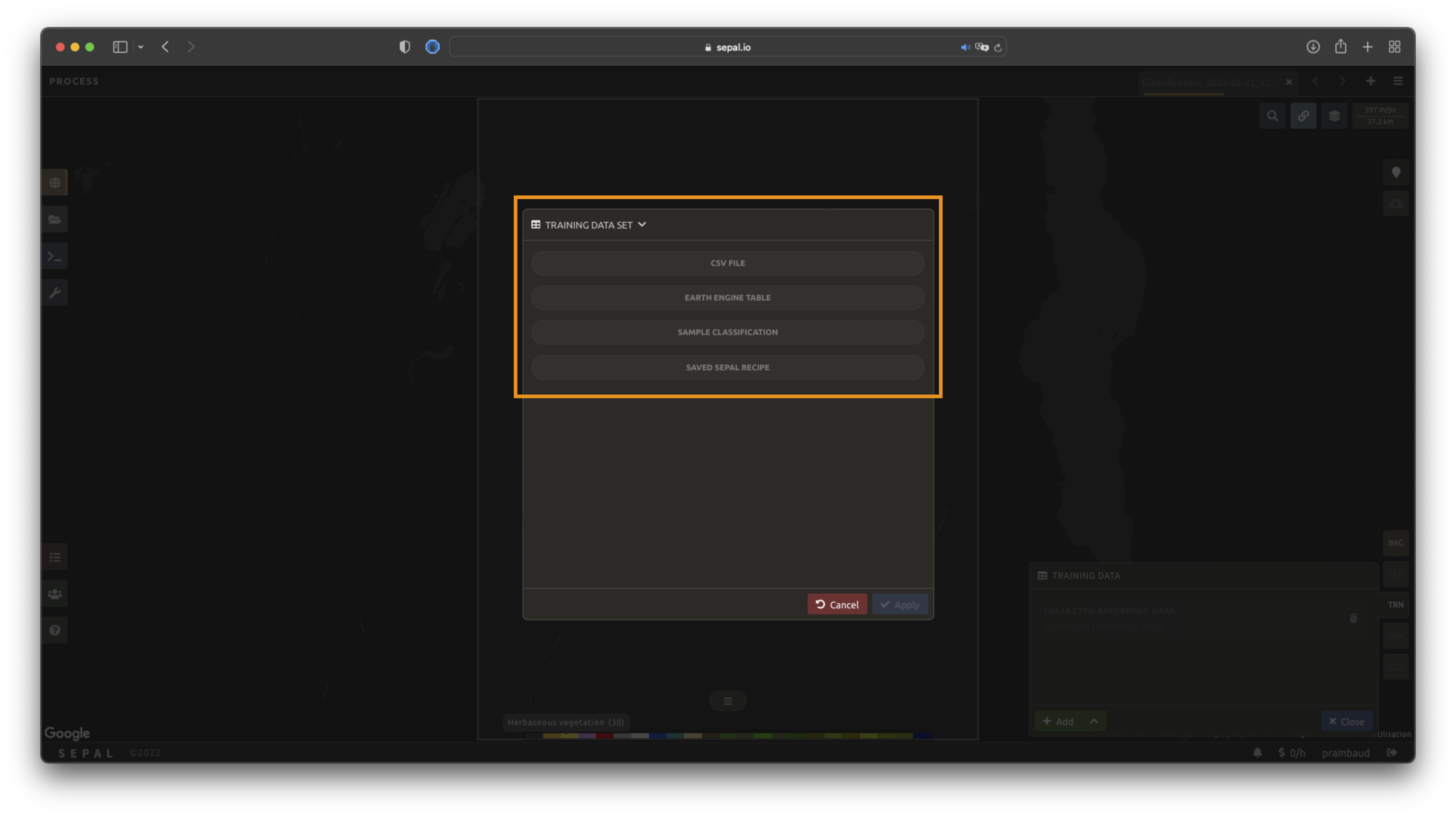
CSV#
By selecting csv file, SEPAL will request a file from your computer in .csv format. The file needs to include two pieces of information: geographic coordinates and class value.
This can be done using coordinates in EPSG:4326 latitude and longitude, as well as a GeoJSON compatible point object. The file can embed other multiple columns that will not be considered during the analysis.
The following table is compatible with SEPAL:
XCoordinate,YCoordinate,class,class_name,editor_name
32.77189961605467,-11.616264558754402,80,Shrublands,Pierrick rambaud
...
The columns used to define the X (longitude) and Y (latitude) coordinates are manually set up in the pop-up window. Select Next once every column is filled.
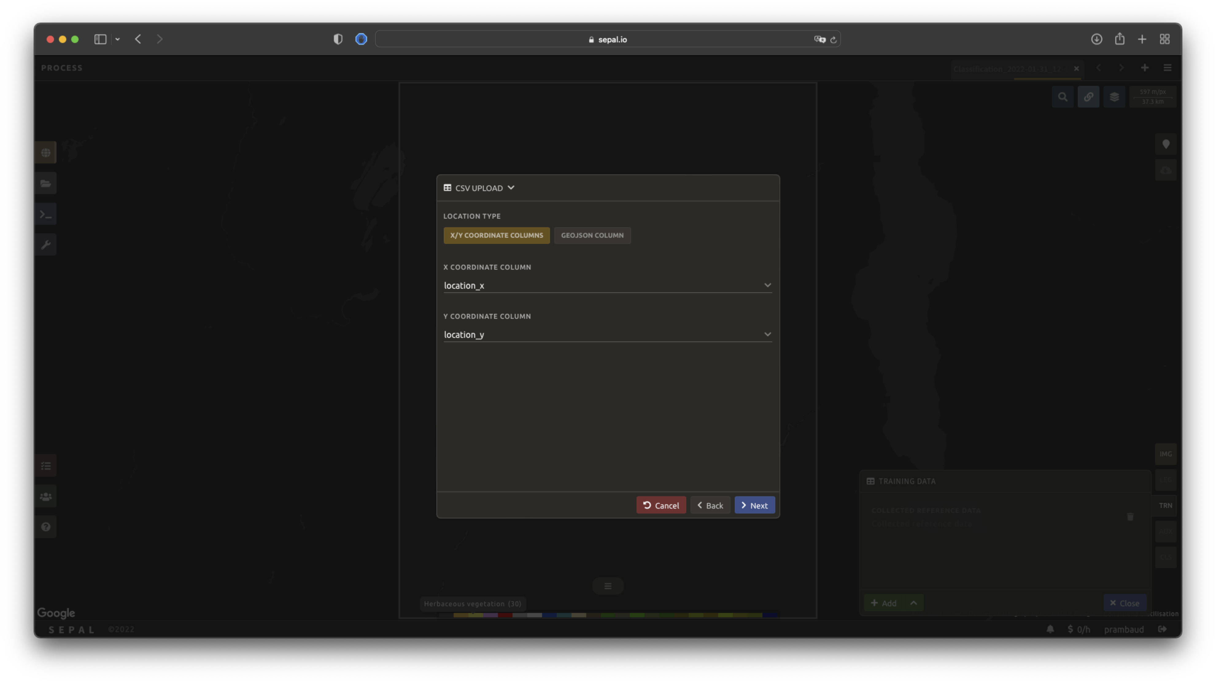
Astuce
If your file contains a GeoJSON column instead of coordinates, select geojson column to switch the interface to one column selection.
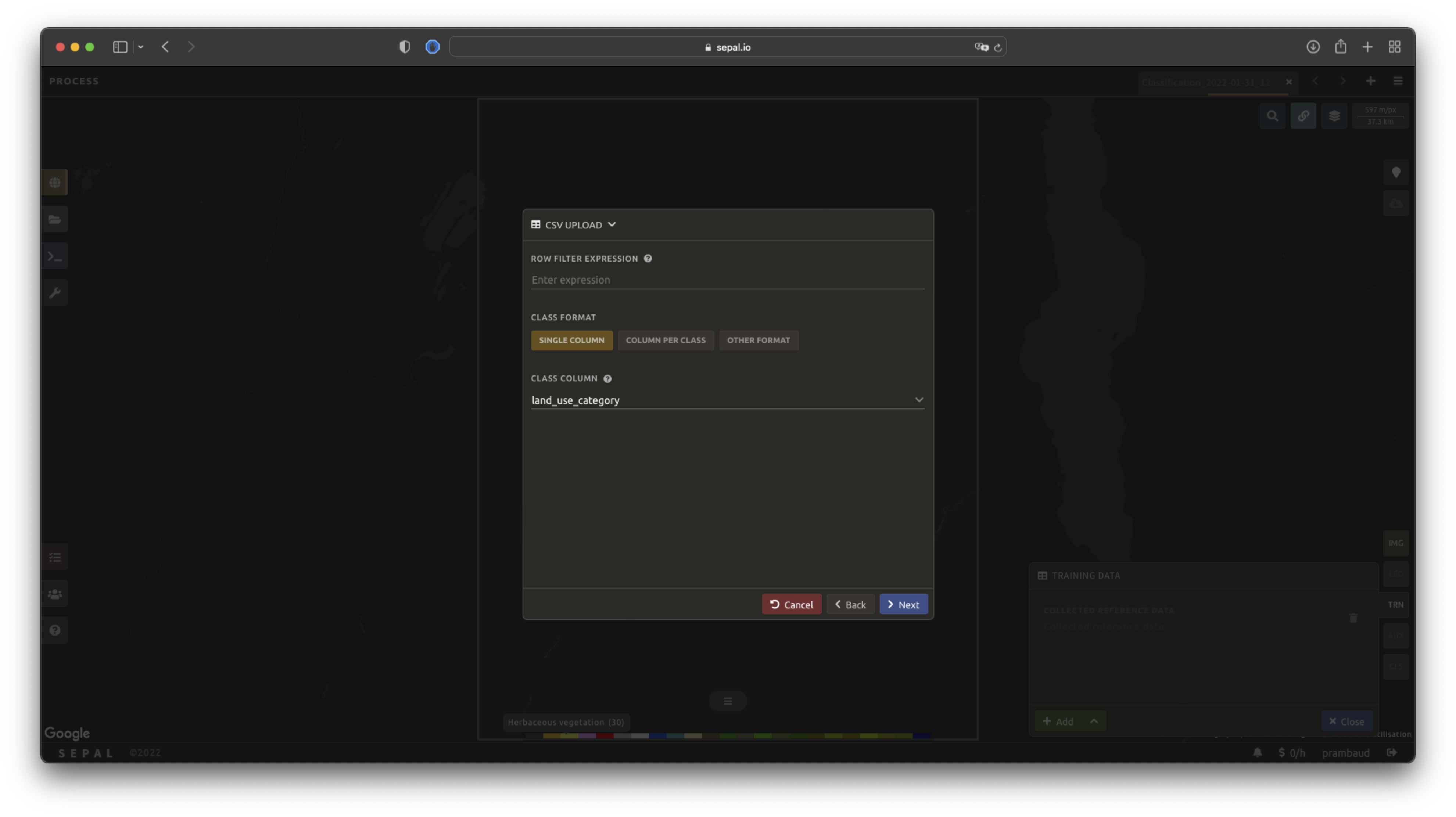
Now that you have set up the coordinates of your points, SEPAL will request the columns specifying the class value (not the name) in a second frame. Only the single column is supported so far. Select the column from your file that embeds the class values.
Astuce
Using the row filter expression text field, one can filter out some lines of the table. Refer to the features section to learn more.
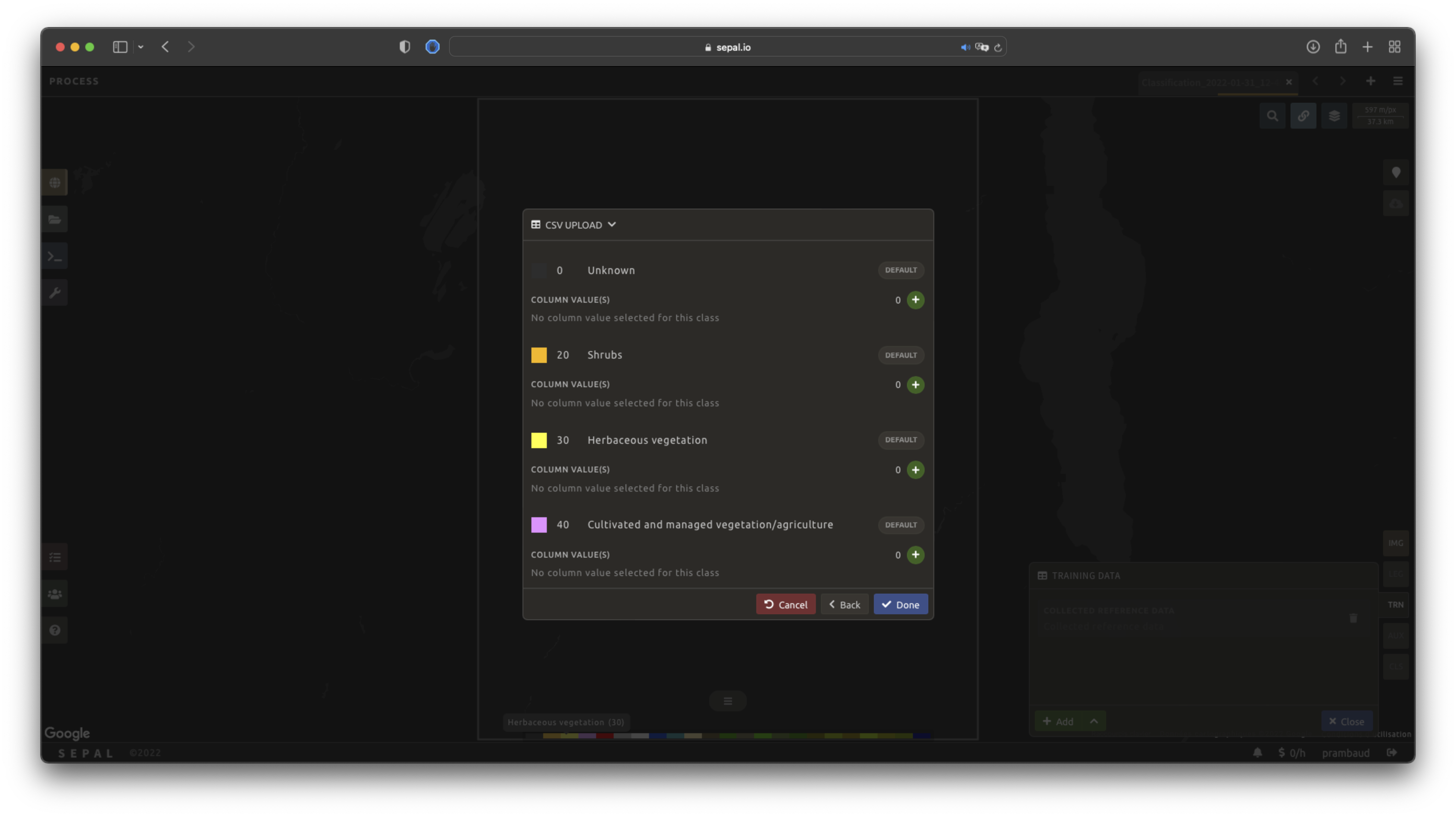
Select next to add the data to the model. SEPAL will provide a summary of the classes in the legend of the classification and the number of training points added by your file.
Selecting the Done button will complete the uploading procedure.
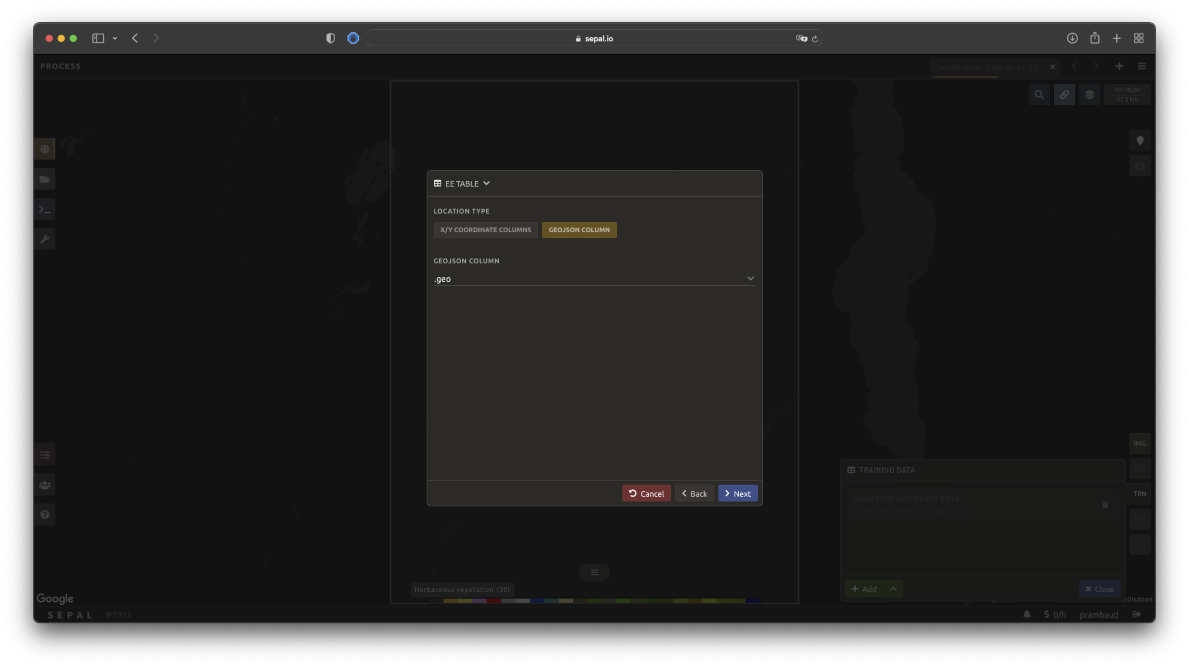
GEE table#
By selecting Earth Engine Table, SEPAL will request a file from your computer in .csv format. The file needs to provide two pieces of information: geographic coordinates and class value.
The process is nearly the same as found in the documentation above discussing .csv tables. The only difference should be the geometry column, as GEE assets usually embed a .goejson column by default. If this column exists, it will be autodetected by SEPAL.
For the other steps, please reproduce what was presented in the .csv section above.
Note
To build the documentation example, use this public asset: projects/sepal-cookbook/assets/classification/zmb_eastern_esa_2012_2021_reference_data.
Sample classification#
Instead of providing dataset points, SEPAL can also extract reference data from an already existing classification – which is a good way to improve an already existing classification system using an image with a better resolution.
To sample data, SEPAL will randomly select a number of points in each class and extract the class value using the provided resolution.
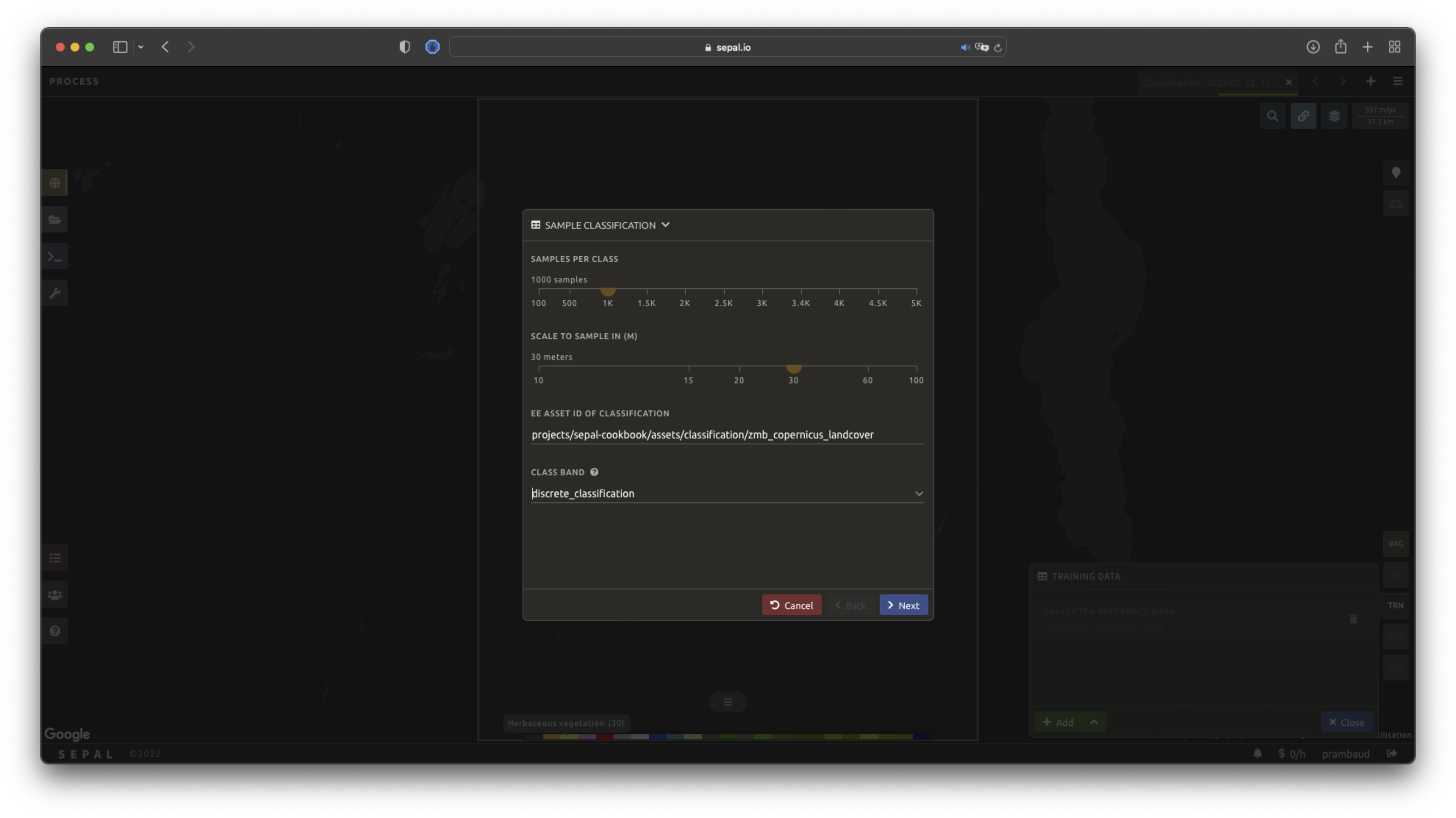
Start by selecting btn:Sample classification in the opened pop-up window, where all of the the parameters can be set:
Sample per class: the number of samples per class of the provided image. The more samples you request, the more accurate the model will be (if too many samples are selected, on-the-fly visualization will never render; default to:
1000).Scale to sample in: the scale used to create the sample in the provided image (it should match the image to classify resolution; default to:
30 m).EE asset ID: the ID of the classification to sample (it should be an
ee.Imageaccessible to the user).Class band: The class to use for classification value (the dropdown menu will be filled with the bands found in the provided asset).
Note
To reproduce this example, use the following asset as an image to sample: projects/sepal-cookbook/assets/classification/zmb_copernicus_landcover.
Note
When all of the parameters are selected, it can take time, as SEPAL builds the sampling values on the fly. They will only be displayed once the sampling is validated.
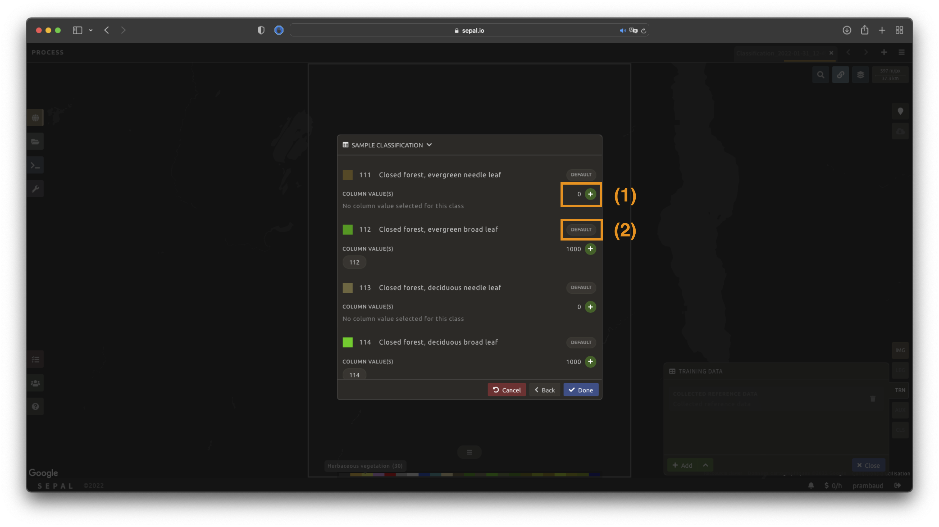
Select Next to display the sampling summary. In this pane, SEPAL displays each class of the legend (as defined in the previous subsection) and the number of samples created for it.
Select the buttons (1) to change the number of samples in a specific class. By default, SEPAL ignores the samples with a Null value. One can select Default (2) for any of the classes so that these points end up in the default class instead of being ignored.
SEPAL recipe#
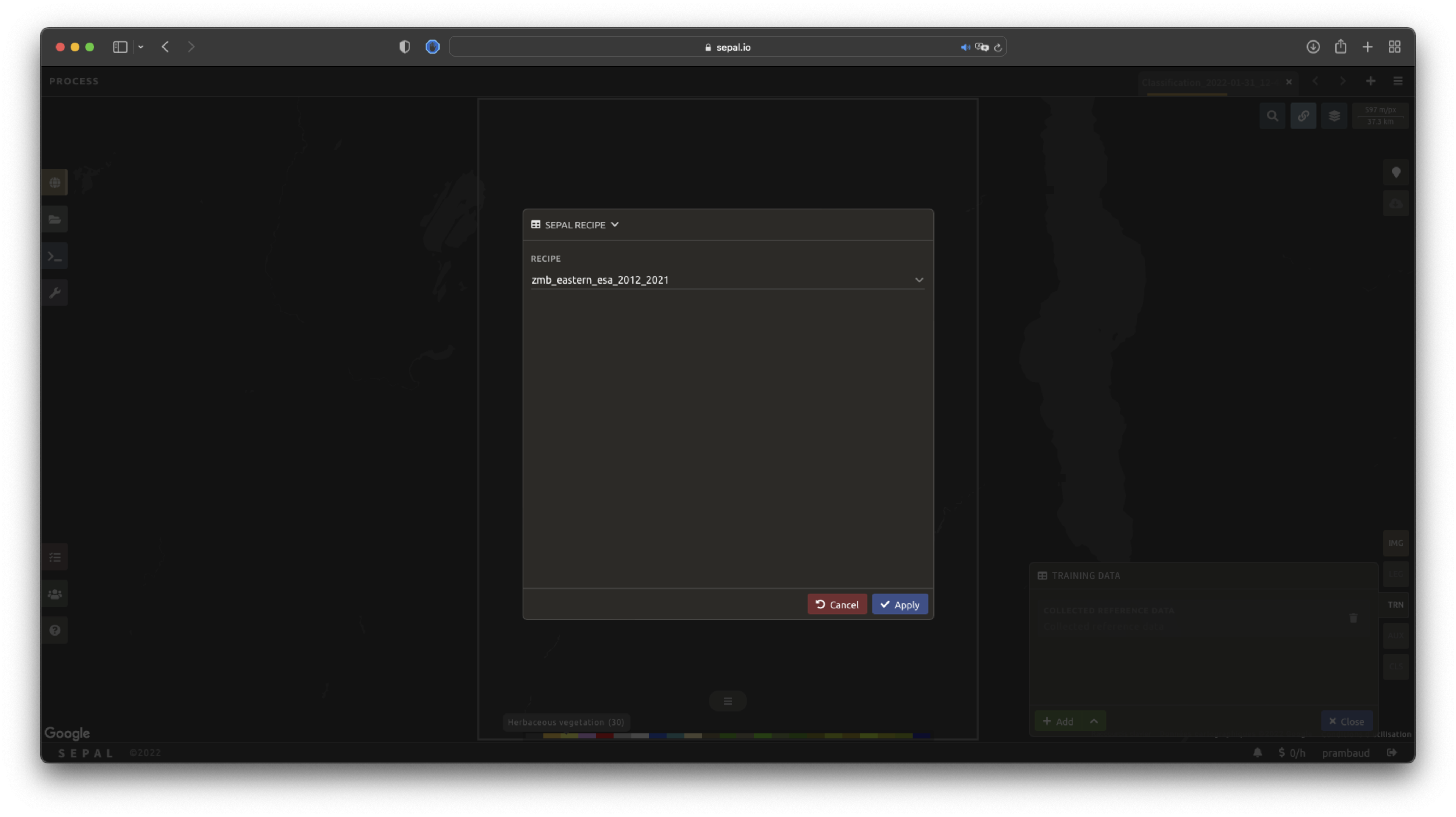
SEPAL is also able to directly apply a model built in another recipe as training data. In this case, we are not importing the points, but all of the model from the external recipe. It will not add points to the map. It’s useful when the same classification needs to be applied on the same area for multiple years. The classification work can be carried out only in the first year and then applied recursively on all the others.
Select Saved SEPAL recipe to open the pop-up window. In the dropdown menu, select one of the recipes saved in your SEPAL account.
Note
The imported recipe needs to be a Classification recipe. If none are found, the dropdown menu will be empty.
This recipe cannot come from another SEPAL account.
Use auxiliary datasets#
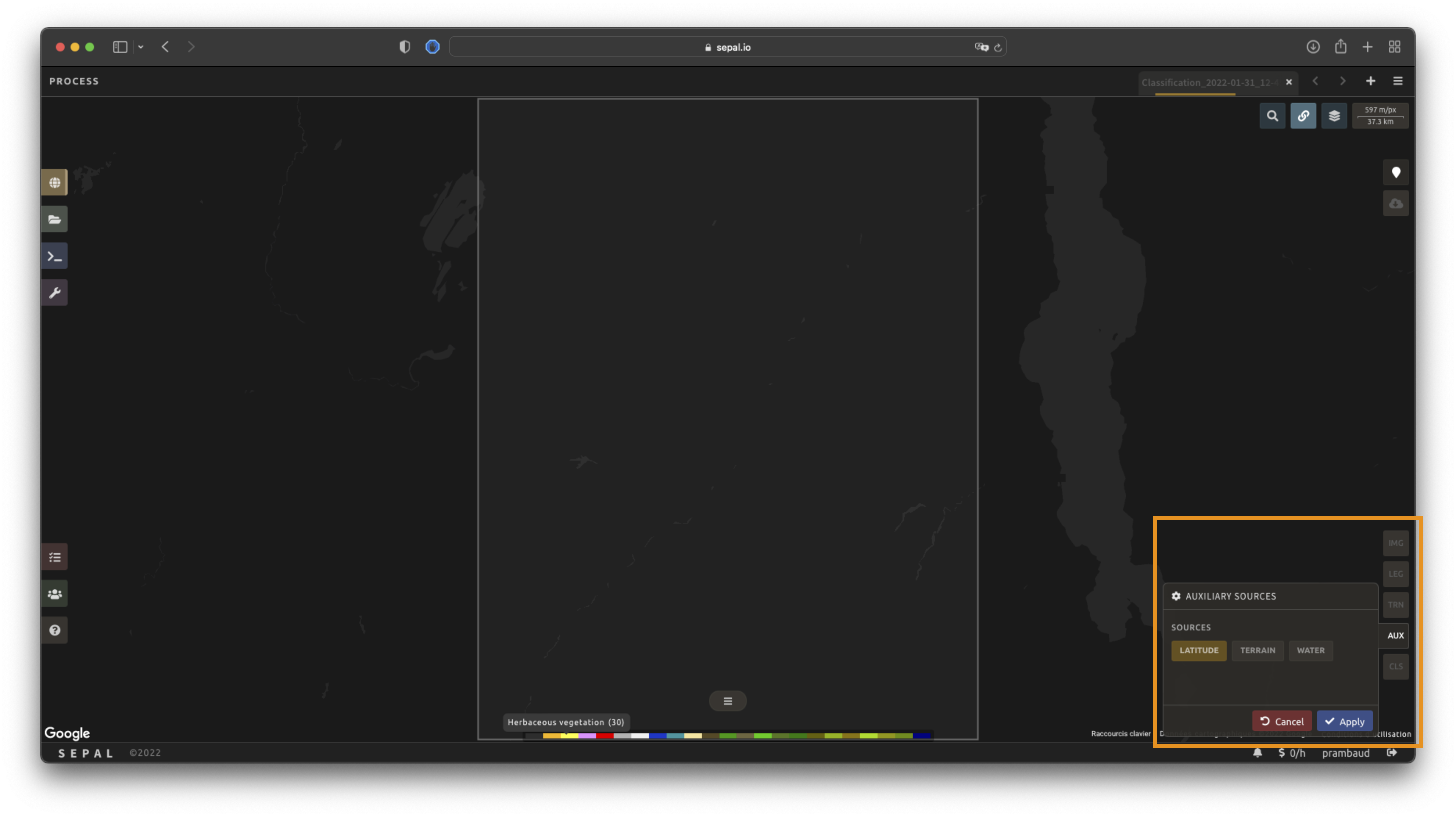
Some information that could be useful to the classification model is not always included in your image bands. A common example is Elevation. In order to improve the quality of the classification, SEPAL can provide some extra datasets to add auxiliary bands to the classification model.
Select AUX to open the Auxiliaries tab. Three sources are currently implemented in the platform (any number of them can be selected):
Latitude: On-the-fly latitude dataset built from the coordinates of each pixel’s center.
Terrain: From the NASA SRTM Digital Elevation 30 m dataset, SEPAL will use the
Elevation,SlopeandAspectbands. It will also add anEastnessandNorthnessband derived fromAspect.Water: From the JRC Global Surface Water Mapping Layers, v1.3 dataset, SEPAL will add the following bands:
occurrence,change_abs,change_norm,seasonality,max_extent,water_occurrence,water_change_abs,water_change_norm,water_seasonalityandwater_max_extent.
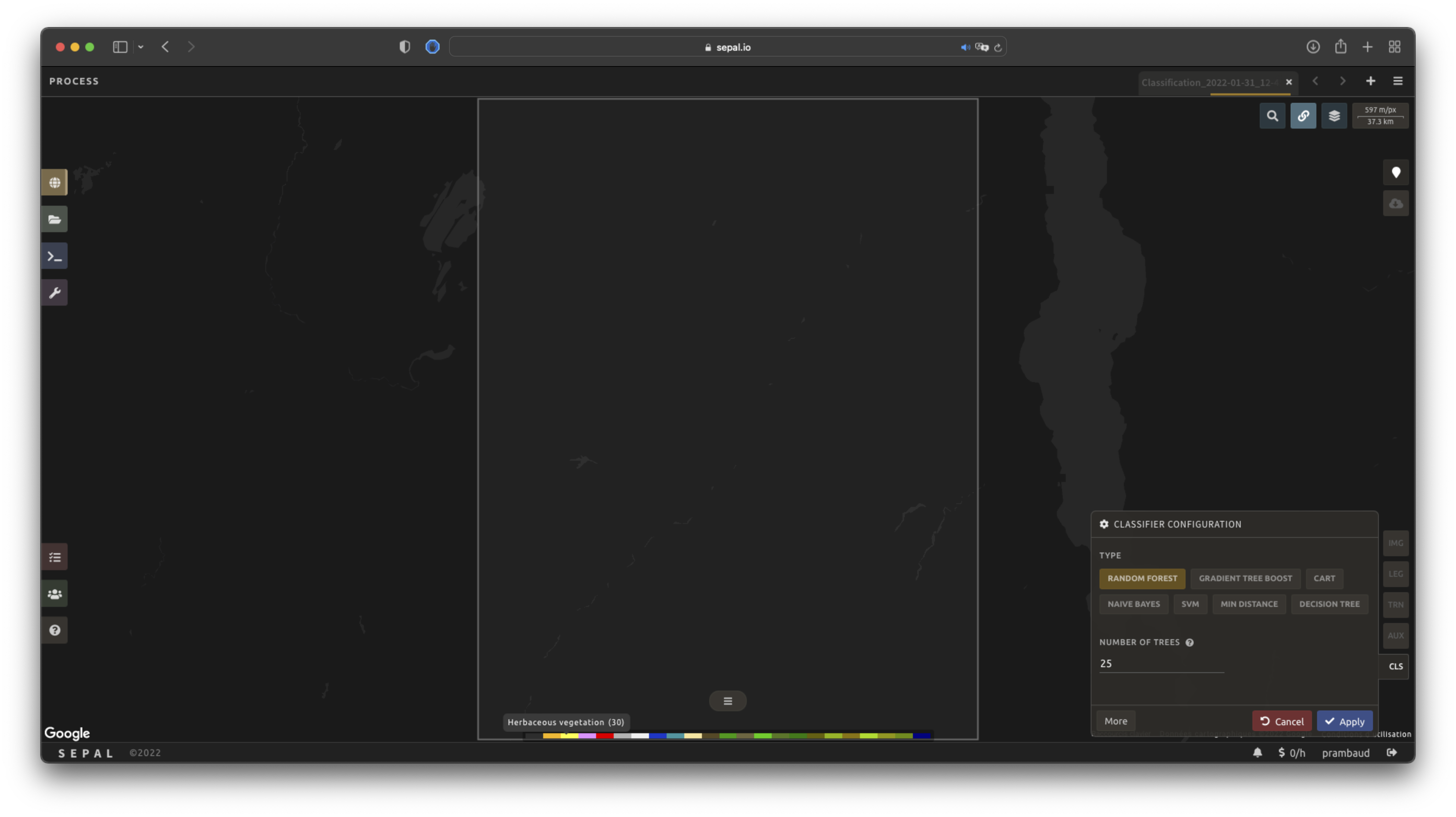
Classifier configuration#
Note
Customizing the classifier is a section designed for advanced users. Make sure that you thoroughly understand how the classifier you’re using works before changing its parameters.
Note
The default value is a Random Forest classifier using 25 trees.
The Classification tool used in SEPAL is based on the Smile - Statistical Machine Intelligence and Learning Engine Javascript library (refer to their documentation for specific descriptions of each model).
Select CLS to open the Classification parameter menu. SEPAL supports seven classifiers:
random forest
gradient tree boost
cart
naive bayes
SVM
min distance
decision tree
For each of them, the workflow is the same:
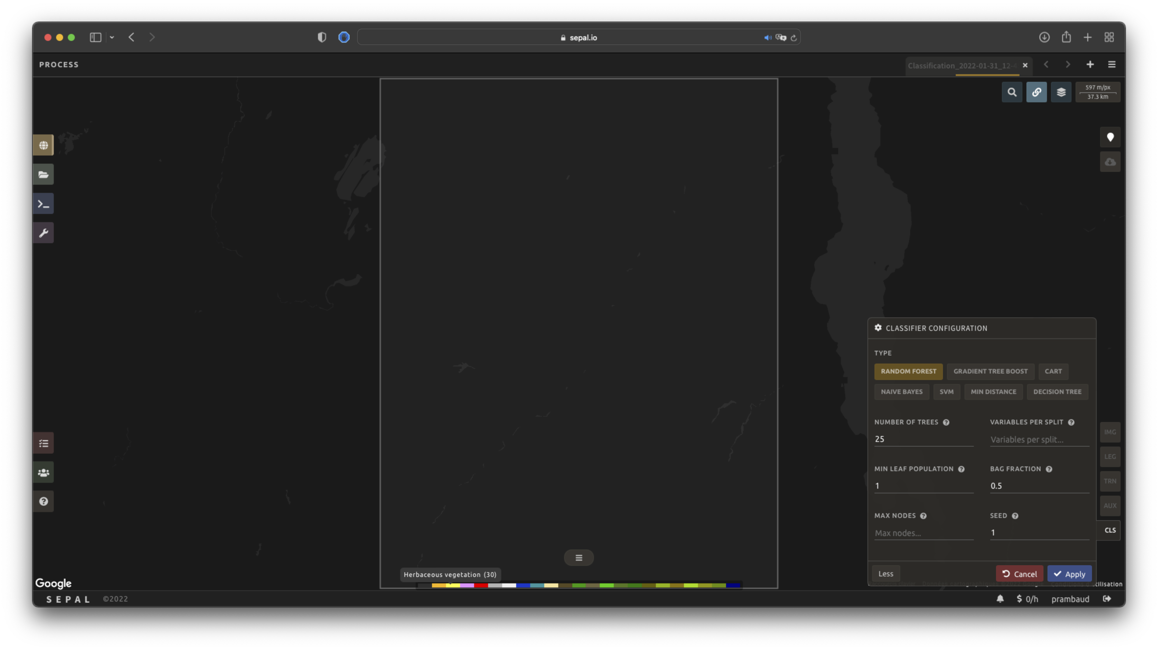
Select the classifier by clicking on the corresponding name. SEPAL will display some of the parameters available.
Select More on the lower-left side of the panel to fully customize your classifier. The classification results will be updated on the fly.
On-the-fly training#
Note
This process requires a good understanding of the Visualization feature of SEPAL (refer to the feature section for more information).
Once all of the parameters are set, the user is free to add extra training data in the web interface and the new points will be added to the final model, improving the quality of the classification.
Set up the view#
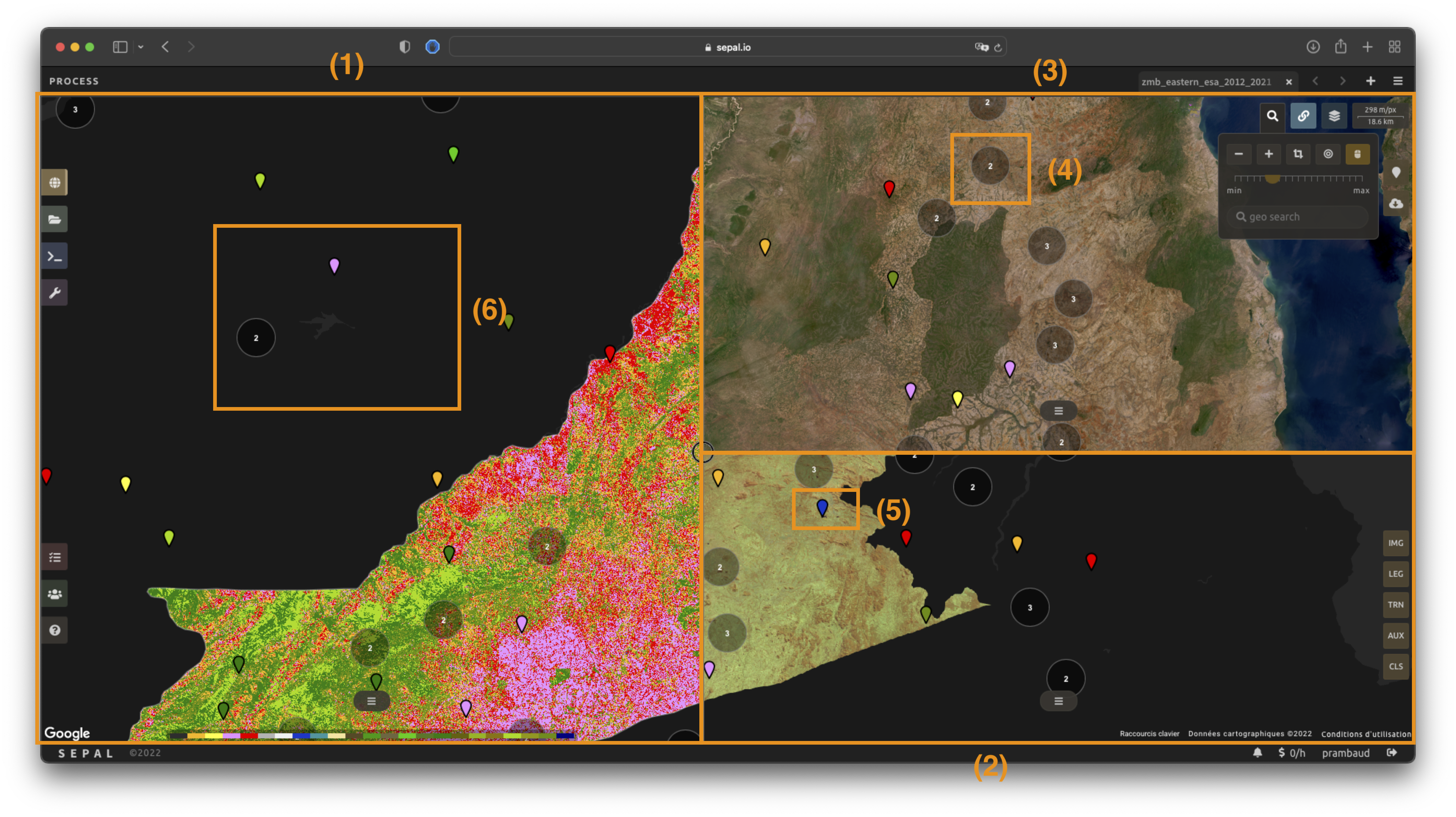
In order to improve the classification, one must set up the view to display all of the information. While these guidelines could be modified and extended, they are still useful as an introductory resource.
In the following image, we displayed:
The current recipe (1) using the class colors in categorical mode.
The current image (what you are classifying) (2) using the NIR,RED,SWIR band combination.
The extra visual dataset NICFI Planet Lab data (3) from 2021.
The number (4) indicates a cluster of existing training points. Zoom in and they will be displayed as markers using the color of the class they mark (5).
Important
This initial classification has been set using sampled data. Since they are sampled from a larger image, some are out of the image. They will have no impact on the classification as they are applied to masked pixels (6).
Select points#
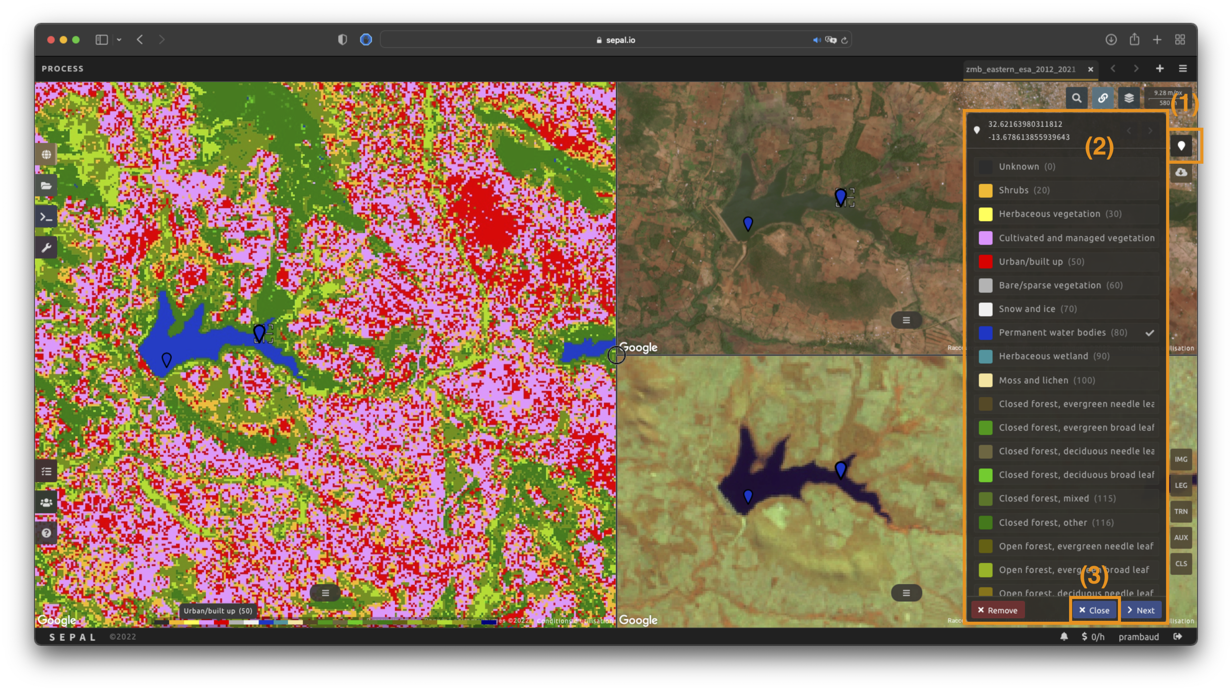
To start adding points, open the training interface by selecting in the upper right of the screen (1). Once selected, the background color becomes darker and the pointer of the mouse becomes a .
The process to add new training data is as follows:
Click on the map to select a point: You can click in any of the panes (not restricted to the Recipe pane), but to be useful, the point needs to be within the border of the AOI. If it’s not already the case, the Class selection panel will appear in the upper right of the window (2).
Select the class value: The previous class value is preselected, but you can change it to any other class value from the defined legend. The legend is displayed as
<legend_classname> (<legend_value>).
You can now click elsewhere on the map to add another point. If you are satisfied with the classification, select Close (3) and select again to stop editing the points. Every time a new point is added, the Classification map is recomputed and rendered on the left side.
Modify existing points#
To modify existing points, select the to open the Point editing interface. Then:
Select a point: To select a point, click on an existing marker. It will appear bolder than the others. If it’s not already the case, the Class selection pane will appear in the upper right.
Change the class value: The point class will be selected in the Editing menu with a . Select any other class value to change it.
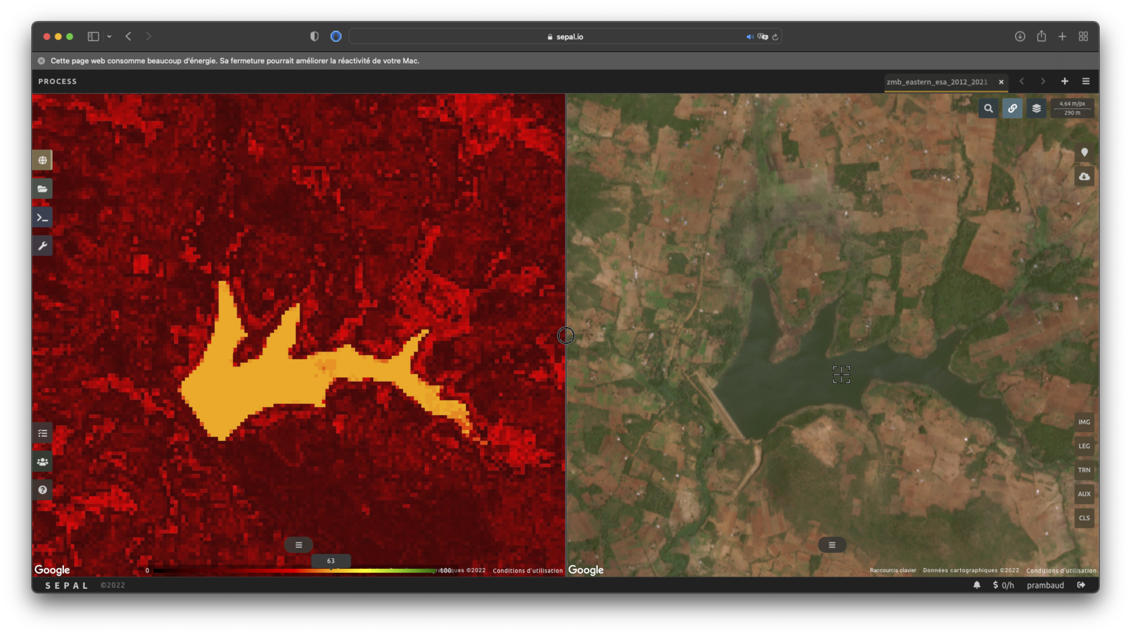
Check the validity#
SEPAL embeds information to help the user understand if the amount of training data is sufficient to produce an accurate classification model. In the Recipe window, change the Band combination to Class probability.
The user now sees the probability of the model (i.e. the confidence level of the level with output class for each pixel).
If the value is high (> 80 percent), then the pixel can be considered valid; if the value is low (< 80 percent), the model needs more training data or extra bands to improve the analysis.
In the example image, the lake is classified as a permanent water body with a confidence of 65 percent, which is higher than the rest of the vegetation around it.
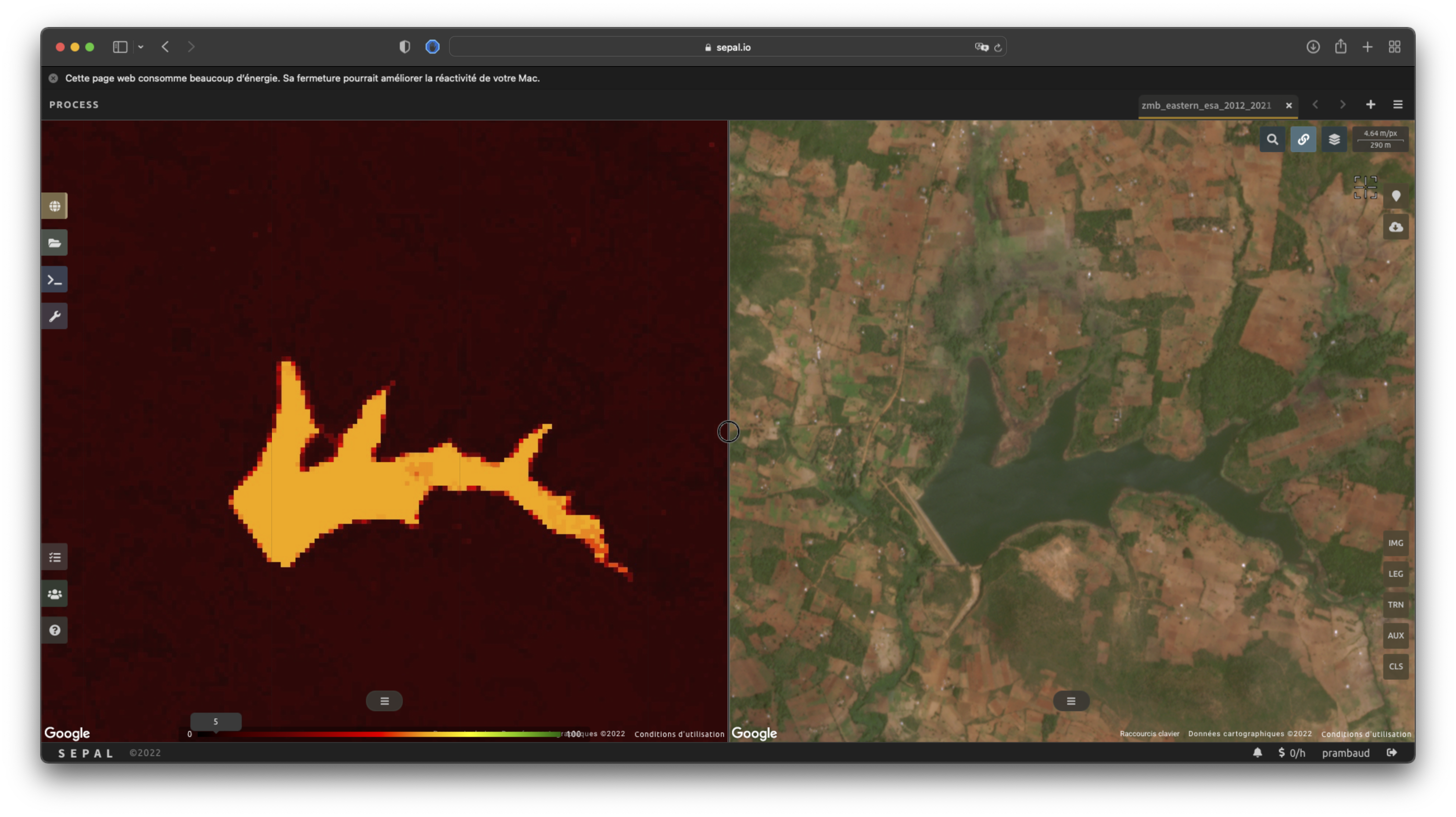
This analysis can also be conducted class-by-class using the built-in <class_name> % bands. Select the one corresponding to the class you want to assess (see the following image) and you’ll get the percentage of confidence for each pixel to be in the sub-mentioned class.
Exporter#
Important
You cannot export a recipe as an asset or a .tiff file without a small computation quota. If you are a new user, see Gérer vos ressources.
Start download#
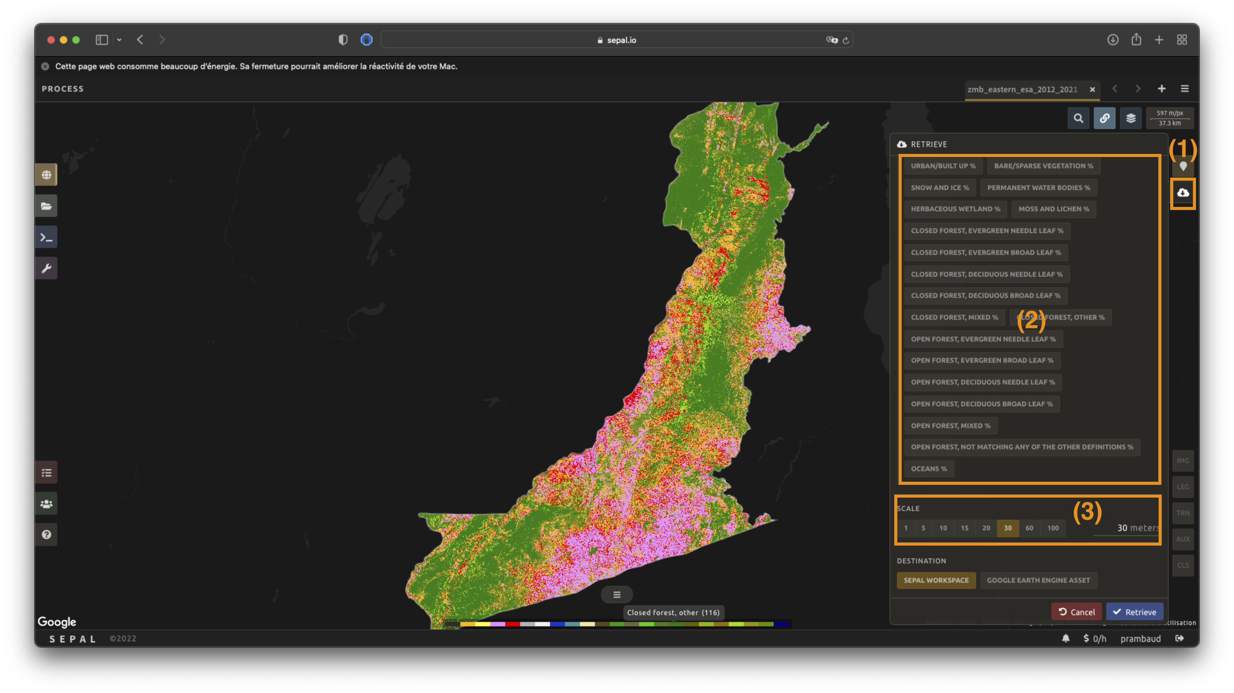
Selecting the tab will open the Retrieve pane, where you can select the exportation parameters (1).
You need to select the band to export (2). There is no maximum number of bands; however, exporting useless bands will only increase the size and time of the output.
You can set a custom scale for exportation (3) by changing the value of the slider in metres (m). (Note: Requesting a smaller resolution than images” native resolution will not improve the quality of the output – just its size; keep in mind that the native resolution of Sentinel data is 10 m, while Landsat is 30 m.)
You can export the image to the SEPAL workspace or to the Google Earth Engine Asset list. The same image will be exported, but for the former, you will find it in .tif format in the Downloads folder; for the latter, the image will be exported to your GEE account asset list.
Note
If Google Earth Engine Asset is not displayed, your GEE account is not connected to SEPAL. Refer to Connect SEPAL to GEE.
Select Apply to start the download process.
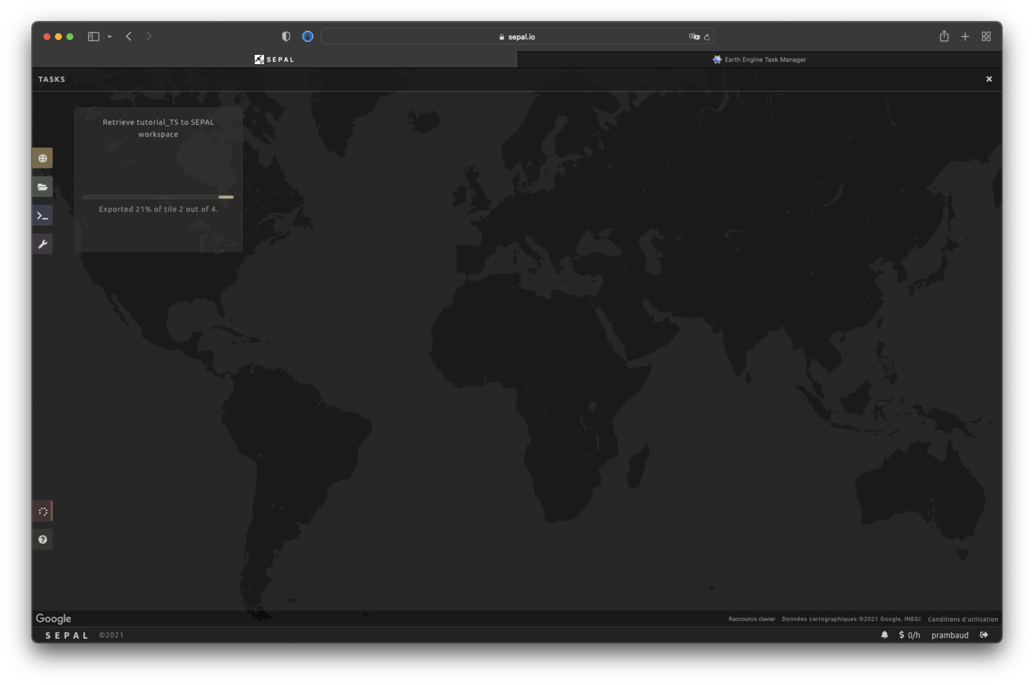
État d’exportation#
By going to the Tasks tab (in the lower-left corner using the or buttons, depending on the loading status), you will see the list of different loading tasks.
The interface will provide you with information about the task progress and display an error if the exportation has failed. If you are unsatisfied with the way we present information, the task can also be monitored using the GEE task manager.
Astuce
This operation is running between GEE and SEPAL servers in the background. You can close the SEPAL page without ending the process.
When the task is finished, the frame will be displayed in green, as shown in the second image below.

Access#
Once the download process is done, you can access the data in your SEPAL folders. The data will be stored in the Downloads folder using the following format:
.
└── downloads/
    └── <CLASSIF name>/
        ├── <CLASSIF name>_<gee tile id>.tif
        ├── <CLASSIF name>_<gee tile id>.tif
        ├── ...
        ├── <CLASSIF name>_<gee tile id>.tif
        └── <CLASSIF name>_<gee tile id>.vrt
Note
Understanding how images are stored in an optical mosaic is only required if you want to manually use them. The SEPAL applications are bound to this tiling system and can digest this information for you.
The data are stored in a folder using the name of the optical mosaic as it was created in the first section of this article. As the data are spatially too big to be exported at once, they are divided into smaller pieces and brought back together in a <MO name>_<gee tile id>.vrt file.
Astuce
The full folder with a consistent tree folder is required to read the .vrt.